Difference between revisions of "Directory:Jon Awbrey/Papers/Differential Logic : Introduction"

Revision as of 16:38, 29 November 2015

Differential logic is the component of logic whose object is the description of variation — for example, the aspects of change, difference, distribution, and diversity — in universes of discourse that are subject to logical description. A definition that broad naturally incorporates any study of variation by way of mathematical models, but differential logic is especially charged with the qualitative aspects of variation that pervade or precede quantitative models. To the extent that a logical inquiry makes use of a formal system, its differential component treats the principles that govern the use of a differential logical calculus, that is, a formal system with the expressive capacity to describe change and diversity in a logical universe of discourse.

A simple example of a differential logical calculus is furnished by a differential propositional calculus. A differential propositional calculus is a propositional calculus extended by a set of terms for describing aspects of change and difference, for example, processes that take place in a universe of discourse or transformations that map a source universe into a target universe. This augments ordinary propositional calculus in the same way that the differential calculus of Leibniz and Newton augments the analytic geometry of Descartes.

Quick Overview

Cactus Language for Propositional Logic

The development of differential logic is greatly facilitated by having a conceptually efficient calculus in place at the level of boolean-valued functions and elementary logical propositions. A calculus that is very efficient from both conceptual and computational standpoints is based on just two types of logical connectives, both of variable $k\!$ -ary scope. The formulas of this calculus map into a species of graph-theoretical structures called painted and rooted cacti (PARCs) that lend visual representation to their functional structure and smooth the path to efficient computation.

The first kind of propositional expression is a parenthesized sequence of propositional expressions, written as $\texttt{(} e_1 \texttt{,} e_2 \texttt{,} \ldots \texttt{,} e_{k-1} \texttt{,} e_k \texttt{)}\!$ and read to say that exactly one of the propositions $e_1, e_2, \ldots, e_{k-1}, e_k\!$ is false, in other words, that their minimal negation is true. A clause of this form maps into a PARC structure called a lobe, in this case, one that is painted with the colors $e_1, e_2, \ldots, e_{k-1}, e_k\!$ as shown below.

The second kind of propositional expression is a concatenated sequence of propositional expressions, written as $e_1\ e_2\ \ldots\ e_{k-1}\ e_k\!$ and read to say that all of the propositions $e_1, e_2, \ldots, e_{k-1}, e_k\!$ are true, in other words, that their logical conjunction is true. A clause of this form maps into a PARC structure called a node, in this case, one that is painted with the colors $e_1, e_2, \ldots, e_{k-1}, e_k\!$ as shown below.

All other propositional connectives can be obtained through combinations of these two forms. Strictly speaking, the parenthesized form is sufficient to define the concatenated form, making the latter formally dispensable, but it is convenient to maintain it as a concise way of expressing more complicated combinations of parenthesized forms. While working with expressions solely in propositional calculus, it is easiest to use plain parentheses for logical connectives. In contexts where ordinary parentheses are needed for other purposes an alternate typeface $\texttt{(} \ldots \texttt{)}\!$ may be used for logical operators.

Table 1 collects a sample of basic propositional forms as expressed in terms of cactus language connectives.

$\text{Table 1.} ~~ \text{Syntax and Semantics of a Calculus for Propositional Logic}\!$
$\text{Expression}~\!$	$\text{Interpretation}\!$	$\text{Other Notations}\!$
	$\text{True}\!$	$1\!$
$\texttt{(~)}\!$	$\text{False}\!$	$0\!$
$x\!$	$x\!$	$x\!$
$\texttt{(} x \texttt{)}\!$	$\text{Not}~ x\!$	$\begin{matrix} x' \\ \tilde{x} \\ \lnot x \end{matrix}\!$
$x~y~z\!$	$x ~\text{and}~ y ~\text{and}~ z\!$	$x \land y \land z\!$
$\texttt{((} x \texttt{)(} y \texttt{)(} z \texttt{))}\!$	$x ~\text{or}~ y ~\text{or}~ z\!$	$x \lor y \lor z\!$
$\texttt{(} x ~ \texttt{(} y \texttt{))}\!$	$\begin{matrix} x ~\text{implies}~ y \\ \mathrm{If}~ x ~\text{then}~ y \end{matrix}$	$x \Rightarrow y\!$
$\texttt{(} x \texttt{,} y \texttt{)}\!$	$\begin{matrix} x ~\text{not equal to}~ y \\ x ~\text{exclusive or}~ y \end{matrix}$	$\begin{matrix} x \ne y \\ x + y \end{matrix}$
$\texttt{((} x \texttt{,} y \texttt{))}\!$	$\begin{matrix} x ~\text{is equal to}~ y \\ x ~\text{if and only if}~ y \end{matrix}$	$\begin{matrix} x = y \\ x \Leftrightarrow y \end{matrix}$
$\texttt{(} x \texttt{,} y \texttt{,} z \texttt{)}\!$	$\begin{matrix} \text{Just one of} \\ x, y, z \\ \text{is false}. \end{matrix}$	$\begin{matrix} x'y~z~ & \lor \\ x~y'z~ & \lor \\ x~y~z' & \end{matrix}$
$\texttt{((} x \texttt{),(} y \texttt{),(} z \texttt{))}\!$	$\begin{matrix} \text{Just one of} \\ x, y, z \\ \text{is true}. \\ & \\ \text{Partition all} \\ \text{into}~ x, y, z. \end{matrix}$	$\begin{matrix} x~y'z' & \lor \\ x'y~z' & \lor \\ x'y'z~ & \end{matrix}$
$\begin{matrix} \texttt{((} x \texttt{,} y \texttt{),} z \texttt{)} \\ & \\ \texttt{(} x \texttt{,(} y \texttt{,} z \texttt{))} \end{matrix}\!$	$\begin{matrix} \text{Oddly many of} \\ x, y, z \\ \text{are true}. \end{matrix}\!$	$x + y + z\!$ $\begin{matrix} x~y~z~ & \lor \\ x~y'z' & \lor \\ x'y~z' & \lor \\ x'y'z~ & \end{matrix}\!$
$\texttt{(} w \texttt{,(} x \texttt{),(} y \texttt{),(} z \texttt{))}\!$	$\begin{matrix} \text{Partition}~ w \\ \text{into}~ x, y, z. \\ & \\ \text{Genus}~ w ~\text{comprises} \\ \text{species}~ x, y, z. \end{matrix}$	$\begin{matrix} w'x'y'z' & \lor \\ w~x~y'z' & \lor \\ w~x'y~z' & \lor \\ w~x'y'z~ & \end{matrix}$

The simplest expression for logical truth is the empty word, usually denoted by $\boldsymbol\varepsilon\!$ or $\lambda\!$ in formal languages, where it forms the identity element for concatenation. To make it visible in context, it may be denoted by the equivalent expression ${}^{\backprime\backprime} \texttt{((~))} {}^{\prime\prime},\!$ or, especially if operating in an algebraic context, by a simple ${}^{\backprime\backprime} 1 {}^{\prime\prime}.\!$ Also when working in an algebraic mode, the plus sign ${}^{\backprime\backprime} + {}^{\prime\prime}\!$ may be used for exclusive disjunction. For example, we have the following paraphrases of algebraic expressions by means of parenthesized expressions:

$\begin{matrix} a + b & = & \texttt{(} a \texttt{,} b \texttt{)} \end{matrix}\!$

$\begin{matrix} a + b + c & = & \texttt{(} a \texttt{,(} b \texttt{,} c \texttt{))} & = & \texttt{((} a \texttt{,} b \texttt{),} c \texttt{)} \end{matrix}\!$

It is important to note that the last expressions are not equivalent to the 3-place parenthesis $\texttt{(} a \texttt{,} b \texttt{,} c \texttt{)}.\!$

Differential Expansions of Propositions

Bird's Eye View

An efficient calculus for the realm of logic represented by boolean functions and elementary propositions makes it feasible to compute the finite differences and the differentials of those functions and propositions.

For example, consider a proposition of the form ${}^{\backprime\backprime} \, p ~\mathrm{and}~ q \, {}^{\prime\prime}\!$ that is graphed as two letters attached to a root node:

Written as a string, this is just the concatenation $p~q\!$ .

The proposition $pq\!$ may be taken as a boolean function $f(p, q)\!$ having the abstract type $f : \mathbb{B} \times \mathbb{B} \to \mathbb{B},\!$ where $\mathbb{B} = \{ 0, 1 \}~\!$ is read in such a way that $0\!$ means $\mathrm{false}\!$ and $1\!$ means $\mathrm{true}.\!$

Imagine yourself standing in a fixed cell of the corresponding venn diagram, say, the cell where the proposition $pq\!$ is true, as shown in the following Figure:

Now ask yourself: What is the value of the proposition $pq\!$ at a distance of $\mathrm{d}p\!$ and $\mathrm{d}q\!$ from the cell $pq\!$ where you are standing?

Don't think about it — just compute:

The cactus formula $\texttt{(p, dp)(q, dq)}\!$ and its corresponding graph arise by substituting $p + \mathrm{d}p\!$ for $p\!$ and $q + \mathrm{d}q\!$ for $q\!$ in the boolean product or logical conjunction $pq\!$ and writing the result in the two dialects of cactus syntax. This follows from the fact that the boolean sum $p + \mathrm{d}p\!$ is equivalent to the logical operation of exclusive disjunction, which parses to a cactus graph of the following form:

Next question: What is the difference between the value of the proposition $pq\!$ over there, at a distance of $\mathrm{d}p\!$ and $\mathrm{d}q,\!$ and the value of the proposition $pq\!$ where you are standing, all expressed in the form of a general formula, of course? Here is the appropriate formulation:

There is one thing that I ought to mention at this point: Computed over $\mathbb{B},\!$ plus and minus are identical operations. This will make the relation between the differential and the integral parts of the appropriate calculus slightly stranger than usual, but we will get into that later.

Last question, for now: What is the value of this expression from your current standpoint, that is, evaluated at the point where $pq\!$ is true? Well, substituting $1\!$ for $p\!$ and $1\!$ for $q\!$ in the graph amounts to erasing the labels $p\!$ and $q\!,\!$ as shown here:

And this is equivalent to the following graph:

We have just met with the fact that the differential of the and is the or of the differentials.

$\begin{matrix} p ~\mathrm{and}~ q & \quad & \xrightarrow{\quad\mathrm{Diff}\quad} & \quad & \mathrm{d}p ~\mathrm{or}~ \mathrm{d}q \end{matrix}\!$

It will be necessary to develop a more refined analysis of that statement directly, but that is roughly the nub of it.

If the form of the above statement reminds you of De Morgan's rule, it is no accident, as differentiation and negation turn out to be closely related operations. Indeed, one can find discussions of logical difference calculus in the Boole–De Morgan correspondence and Peirce also made use of differential operators in a logical context, but the exploration of these ideas has been hampered by a number of factors, not the least of which has been the lack of a syntax that was adequate to handle the complexity of expressions that evolve.

Worm's Eye View

Let's run through the initial example again, this time attempting to interpret the formulas that develop at each stage along the way. We begin with a proposition or a boolean function $f(p, q) = pq.\!$

A function like this has an abstract type and a concrete type. The abstract type is what we invoke when we write things like $f : \mathbb{B} \times \mathbb{B} \to \mathbb{B}\!$ or $f : \mathbb{B}^2 \to \mathbb{B}.\!$ The concrete type takes into account the qualitative dimensions or the “units” of the case, which can be explained as follows.

Let

$P\!$ be the set of values

$\{ \texttt{(} p \texttt{)},~ p \} ~=~ \{ \mathrm{not}~ p,~ p \} ~\cong~ \mathbb{B}.\!$

Let

$Q\!$ be the set of values

$\{ \texttt{(} q \texttt{)},~ q \} ~=~ \{ \mathrm{not}~ q,~ q \} ~\cong~ \mathbb{B}.\!$

Then interpret the usual propositions about $p, q\!$ as functions of the concrete type $f : P \times Q \to \mathbb{B}.\!$

We are going to consider various operators on these functions. Here, an operator $\mathrm{F}\!$ is a function that takes one function $f\!$ into another function $\mathrm{F}f.\!$

The first couple of operators that we need to consider are logical analogues of the pair that play a founding role in the classical finite difference calculus, namely:

The difference operator

$\Delta,\!$ written here as

$\mathrm{D}.\!$

The enlargement operator

$\Epsilon,\!$ written here as

$\mathrm{E}.\!$

These days, $\mathrm{E}\!$ is more often called the shift operator.

In order to describe the universe in which these operators operate, it is necessary to enlarge the original universe of discourse. Starting from the initial space $X = P \times Q,\!$ its (first order) differential extension $\mathrm{E}X\!$ is constructed according to the following specifications:

$\begin{array}{rcc} \mathrm{E}X & = & X \times \mathrm{d}X \end{array}\!$

where:

$\begin{array}{rcc} X & = & P \times Q \'"`UNIQ-MathJax1-QINU`"' Amazing! {| align="center" cellpadding="0" cellspacing="0" width="90%" | <p>Consider what effects that might ''conceivably'' have practical bearings you ''conceive'' the objects of your ''conception'' to have. Then, your ''conception'' of those effects is the whole of your ''conception'' of the object.</p> |- | align="right" | — Charles Sanders Peirce, “Issues of Pragmaticism”, (CP 5.438) |} One other subject that it would be opportune to mention at this point, while we have an object example of a mathematical group fresh in mind, is the relationship between the pragmatic maxim and what are commonly known in mathematics as ''representation principles''. As it turns out, with regard to its formal characteristics, the pragmatic maxim unites the aspects of a representation principle with the attributes of what would ordinarily be known as a ''closure principle''. We will consider the form of closure that is invoked by the pragmatic maxim on another occasion, focusing here and now on the topic of group representations. Let us return to the example of the ''four-group'' \(V_4.\!$ We encountered this group in one of its concrete representations, namely, as a transformation group that acts on a set of objects, in this case a set of sixteen functions or propositions. Forgetting about the set of objects that the group transforms among themselves, we may take the abstract view of the group's operational structure, for example, in the form of the group operation table copied here:

$\cdot\!$	$\mathrm{e}\!$	$\mathrm{f}\!$	$\mathrm{g}\!$	$\mathrm{h}\!$
$\mathrm{e}\!$	$\mathrm{e}\!$	$\mathrm{f}\!$	$\mathrm{g}\!$	$\mathrm{h}\!$
$\mathrm{f}\!$	$\mathrm{f}\!$	$\mathrm{e}\!$	$\mathrm{h}\!$	$\mathrm{g}\!$
$\mathrm{g}\!$	$\mathrm{g}\!$	$\mathrm{h}\!$	$\mathrm{e}\!$	$\mathrm{f}\!$
$\mathrm{h}\!$	$\mathrm{h}\!$	$\mathrm{g}\!$	$\mathrm{f}\!$	$\mathrm{e}\!$

This table is abstractly the same as, or isomorphic to, the versions with the $\mathrm{E}_{ij}\!$ operators and the $\mathrm{T}_{ij}\!$ transformations that we took up earlier. That is to say, the story is the same, only the names have been changed. An abstract group can have a variety of significantly and superficially different representations. But even after we have long forgotten the details of any particular representation there is a type of concrete representations, called regular representations, that are always readily available, as they can be generated from the mere data of the abstract operation table itself.

To see how a regular representation is constructed from the abstract operation table, select a group element from the top margin of the Table, and “consider its effects” on each of the group elements as they are listed along the left margin. We may record these effects as Peirce usually did, as a logical aggregate of elementary dyadic relatives, that is, as a logical disjunction or boolean sum whose terms represent the ordered pairs of $\mathrm{input} : \mathrm{output}\!$ transactions that are produced by each group element in turn. This forms one of the two possible regular representations of the group, in this case the one that is called the post-regular representation or the right regular representation. It has long been conventional to organize the terms of this logical aggregate in the form of a matrix:

Reading “ $+\!$ ” as a logical disjunction:

$\begin{matrix} \mathrm{G} & = & \mathrm{e} & + & \mathrm{f} & + & \mathrm{g} & + & \mathrm{h} \end{matrix}\!$

And so, by expanding effects, we get:

$\begin{matrix} \mathrm{G} & = & \mathrm{e}:\mathrm{e} & + & \mathrm{f}:\mathrm{f} & + & \mathrm{g}:\mathrm{g} & + & \mathrm{h}:\mathrm{h} \'"`UNIQ-MathJax2-QINU`"' is the relate, \(j\!$ is the correlate, and in our current example $i\!:\!j,\!$ or more exactly, $m_{ij} = 1,\!$ is taken to say that $i\!$ is a marker for $j.\!$ This is the mode of reading that we call “multiplying on the left”.

In the algebraic, permutational, or transformational contexts of application, however, Peirce converts to the alternative mode of reading, although still calling $i\!$ the relate and $j\!$ the correlate, the elementary relative $i\!:\!j\!$ now means that $i\!$ gets changed into $j.\!$ In this scheme of reading, the transformation $a\!:\!b + b\!:\!c + c\!:\!a\!$ is a permutation of the aggregate $\mathbf{1} = a + b + c,\!$ or what we would now call the set $\{ a, b, c \},\!$ in particular, it is the permutation that is otherwise notated as follows:

$\begin{Bmatrix} a & b & c \\ b & c & a \end{Bmatrix}\!$

This is consistent with the convention that Peirce uses in the paper “On a Class of Multiple Algebras” (CP 3.324–327).

We've been exploring the applications of a certain technique for clarifying abstruse concepts, a rough-cut version of the pragmatic maxim that I've been accustomed to refer to as the operationalization of ideas. The basic idea is to replace the question of What it is, which modest people comprehend is far beyond their powers to answer definitively any time soon, with the question of What it does, which most people know at least a modicum about.

In the case of regular representations of groups we found a non-plussing surplus of answers to sort our way through. So let us track back one more time to see if we can learn any lessons that might carry over to more realistic cases.

Here is is the operation table of $V_4\!$ once again:

$\text{Klein Four-Group}~ V_4\!$
$\cdot\!$	$\mathrm{e}\!$	$\mathrm{f}\!$	$\mathrm{g}\!$	$\mathrm{h}\!$
$\mathrm{e}\!$	$\mathrm{e}\!$	$\mathrm{f}\!$	$\mathrm{g}\!$	$\mathrm{h}\!$
$\mathrm{f}\!$	$\mathrm{f}\!$	$\mathrm{e}\!$	$\mathrm{h}\!$	$\mathrm{g}\!$
$\mathrm{g}\!$	$\mathrm{g}\!$	$\mathrm{h}\!$	$\mathrm{e}\!$	$\mathrm{f}\!$
$\mathrm{h}\!$	$\mathrm{h}\!$	$\mathrm{g}\!$	$\mathrm{f}\!$	$\mathrm{e}\!$

A group operation table is really just a device for recording a certain 3-adic relation, to be specific, the set of triples of the form $(x, y, z)\!$ satisfying the equation $x \cdot y = z.\!$

In the case of $V_4 = (G, \cdot),\!$ where $G\!$ is the underlying set $\{ \mathrm{e}, \mathrm{f}, \mathrm{g}, \mathrm{h} \},\!$ we have the 3-adic relation $L(V_4) \subseteq G \times G \times G\!$ whose triples are listed below:

$\begin{matrix} (\mathrm{e}, \mathrm{e}, \mathrm{e}) & (\mathrm{e}, \mathrm{f}, \mathrm{f}) & (\mathrm{e}, \mathrm{g}, \mathrm{g}) & (\mathrm{e}, \mathrm{h}, \mathrm{h}) \\[6pt] (\mathrm{f}, \mathrm{e}, \mathrm{f}) & (\mathrm{f}, \mathrm{f}, \mathrm{e}) & (\mathrm{f}, \mathrm{g}, \mathrm{h}) & (\mathrm{f}, \mathrm{h}, \mathrm{g}) \\[6pt] (\mathrm{g}, \mathrm{e}, \mathrm{g}) & (\mathrm{g}, \mathrm{f}, \mathrm{h}) & (\mathrm{g}, \mathrm{g}, \mathrm{e}) & (\mathrm{g}, \mathrm{h}, \mathrm{f}) \\[6pt] (\mathrm{h}, \mathrm{e}, \mathrm{h}) & (\mathrm{h}, \mathrm{f}, \mathrm{g}) & (\mathrm{h}, \mathrm{g}, \mathrm{f}) & (\mathrm{h}, \mathrm{h}, \mathrm{e}) \end{matrix}\!$

It is part of the definition of a group that the 3-adic relation $L \subseteq G^3\!$ is actually a function $L : G \times G \to G.\!$ It is from this functional perspective that we can see an easy way to derive the two regular representations. Since we have a function of the type $L : G \times G \to G,\!$ we can define a couple of substitution operators:

1.	$\mathrm{Sub}(x, (\underline{~~}, y))\!$ puts any specified $x\!$ into the empty slot of the rheme $(\underline{~~}, y),\!$ with the effect of producing the saturated rheme $(x, y)\!$ that evaluates to $xy.~\!$
2.	$\mathrm{Sub}(x, (y, \underline{~~}))\!$ puts any specified $x\!$ into the empty slot of the rheme $(y, \underline{~~}),\!$ with the effect of producing the saturated rheme $(y, x)\!$ that evaluates to $yx.~\!$

In (1) we consider the effects of each $x\!$ in its practical bearing on contexts of the form $(\underline{~~}, y),\!$ as $y\!$ ranges over $G,\!$ and the effects are such that $x\!$ takes $(\underline{~~}, y)\!$ into $xy,\!$ for $y\!$ in $G,\!$ all of which is notated as $x = \{ (y : xy) ~|~ y \in G \}.\!$ The pairs $(y : xy)\!$ can be found by picking an $x\!$ from the left margin of the group operation table and considering its effects on each $y\!$ in turn as these run across the top margin. This aspect of pragmatic definition we recognize as the regular ante-representation:

$\begin{matrix} \mathrm{e} & = & \mathrm{e}\!:\!\mathrm{e} & + & \mathrm{f}\!:\!\mathrm{f} & + & \mathrm{g}\!:\!\mathrm{g} & + & \mathrm{h}\!:\!\mathrm{h} \\[4pt] \mathrm{f} & = & \mathrm{e}\!:\!\mathrm{f} & + & \mathrm{f}\!:\!\mathrm{e} & + & \mathrm{g}\!:\!\mathrm{h} & + & \mathrm{h}\!:\!\mathrm{g} \\[4pt] \mathrm{g} & = & \mathrm{e}\!:\!\mathrm{g} & + & \mathrm{f}\!:\!\mathrm{h} & + & \mathrm{g}\!:\!\mathrm{e} & + & \mathrm{h}\!:\!\mathrm{f} \\[4pt] \mathrm{h} & = & \mathrm{e}\!:\!\mathrm{h} & + & \mathrm{f}\!:\!\mathrm{g} & + & \mathrm{g}\!:\!\mathrm{f} & + & \mathrm{h}\!:\!\mathrm{e} \end{matrix}\!$

In (2) we consider the effects of each $x\!$ in its practical bearing on contexts of the form $(y, \underline{~~}),\!$ as $y\!$ ranges over $G,\!$ and the effects are such that $x\!$ takes $(y, \underline{~~})\!$ into $yx,\!$ for $y\!$ in $G,\!$ all of which is notated as $x = \{ (y : yx) ~|~ y \in G \}.\!$ The pairs $(y : yx)\!$ can be found by picking an $x\!$ from the top margin of the group operation table and considering its effects on each $y\!$ in turn as these run down the left margin. This aspect of pragmatic definition we recognize as the regular post-representation:

$\begin{matrix} \mathrm{e} & = & \mathrm{e}\!:\!\mathrm{e} & + & \mathrm{f}\!:\!\mathrm{f} & + & \mathrm{g}\!:\!\mathrm{g} & + & \mathrm{h}\!:\!\mathrm{h} \\[4pt] \mathrm{f} & = & \mathrm{e}\!:\!\mathrm{f} & + & \mathrm{f}\!:\!\mathrm{e} & + & \mathrm{g}\!:\!\mathrm{h} & + & \mathrm{h}\!:\!\mathrm{g} \\[4pt] \mathrm{g} & = & \mathrm{e}\!:\!\mathrm{g} & + & \mathrm{f}\!:\!\mathrm{h} & + & \mathrm{g}\!:\!\mathrm{e} & + & \mathrm{h}\!:\!\mathrm{f} \\[4pt] \mathrm{h} & = & \mathrm{e}\!:\!\mathrm{h} & + & \mathrm{f}\!:\!\mathrm{g} & + & \mathrm{g}\!:\!\mathrm{f} & + & \mathrm{h}\!:\!\mathrm{e} \end{matrix}\!$

If the ante-rep looks the same as the post-rep, now that I'm writing them in the same dialect, that is because $V_4\!$ is abelian (commutative), and so the two representations have the very same effects on each point of their bearing.

So long as we're in the neighborhood, we might as well take in some more of the sights, for instance, the smallest example of a non-abelian (non-commutative) group. This is a group of six elements, say, $G = \{ \mathrm{e}, \mathrm{f}, \mathrm{g}, \mathrm{h}, \mathrm{i}, \mathrm{j} \},\!$ with no relation to any other employment of these six symbols being implied, of course, and it can be most easily represented as the permutation group on a set of three letters, say, $X = \{ a, b, c \},\!$ usually notated as $G = \mathrm{Sym}(X)\!$ or more abstractly and briefly, as $\mathrm{Sym}(3)\!$ or $S_3.\!$ The next Table shows the intended correspondence between abstract group elements and the permutation or substitution operations in $\mathrm{Sym}(X).\!$

$\text{Permutation Substitutions in}~ \mathrm{Sym} \{ a, b, c \}\!$
$\mathrm{e}\!$	$\mathrm{f}\!$	$\mathrm{g}\!$	$\mathrm{h}\!$	$\mathrm{i}~\!$	$\mathrm{j}\!$
$\begin{matrix} a & b & c \\[3pt] \downarrow & \downarrow & \downarrow \\[6pt] a & b & c \end{matrix}\!$	$\begin{matrix} a & b & c \\[3pt] \downarrow & \downarrow & \downarrow \\[6pt] c & a & b \end{matrix}\!$	$\begin{matrix} a & b & c \\[3pt] \downarrow & \downarrow & \downarrow \\[6pt] b & c & a \end{matrix}\!$	$\begin{matrix} a & b & c \\[3pt] \downarrow & \downarrow & \downarrow \\[6pt] a & c & b \end{matrix}\!$	$\begin{matrix} a & b & c \\[3pt] \downarrow & \downarrow & \downarrow \\[6pt] c & b & a \end{matrix}\!$	$\begin{matrix} a & b & c \\[3pt] \downarrow & \downarrow & \downarrow \\[6pt] b & a & c \end{matrix}\!$

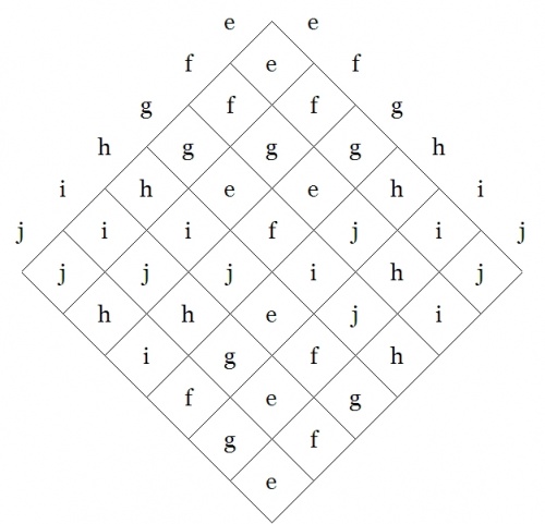
Here is the operation table for $S_3,\!$ given in abstract fashion:

$\text{Symmetric Group}~ S_3\!$

By the way, we will meet with the symmetric group $S_3~\!$ again when we return to take up the study of Peirce's early paper “On a Class of Multiple Algebras” (CP 3.324–327), and also his late unpublished work “The Simplest Mathematics” (1902) (CP 4.227–323), with particular reference to the section that treats of “Trichotomic Mathematics” (CP 4.307–323).

By way of collecting a short-term pay-off for all the work that we did on the regular representations of the Klein 4-group $V_4,\!$ let us write out as quickly as possible in relative form a minimal budget of representations for the symmetric group on three letters, $\mathrm{Sym}(3).\!$ After doing the usual bit of compare and contrast among the various representations, we will have enough concrete material beneath our abstract belts to tackle a few of the presently obscured details of Peirce's early “Algebra + Logic” papers.

Writing the permutations or substitutions of $\mathrm{Sym} \{ a, b, c \}\!$ in relative form generates what is generally thought of as a natural representation of $S_3.~\!$

$\begin{matrix} \mathrm{e} & = & a\!:\!a & + & b\!:\!b & + & c\!:\!c \\[4pt] \mathrm{f} & = & a\!:\!c & + & b\!:\!a & + & c\!:\!b \\[4pt] \mathrm{g} & = & a\!:\!b & + & b\!:\!c & + & c\!:\!a \\[4pt] \mathrm{h} & = & a\!:\!a & + & b\!:\!c & + & c\!:\!b \\[4pt] \mathrm{i} & = & a\!:\!c & + & b\!:\!b & + & c\!:\!a \\[4pt] \mathrm{j} & = & a\!:\!b & + & b\!:\!a & + & c\!:\!c \end{matrix}\!$

I have without stopping to think about it written out this natural representation of $S_3~\!$ in the style that comes most naturally to me, to wit, the “right” way, whereby an ordered pair configured as $x\!:\!y\!$ constitutes the turning of $x\!$ into $y.\!$ It is possible that the next time we check in with CSP we will have to adjust our sense of direction, but that will be an easy enough bridge to cross when we come to it.

To construct the regular representations of $S_3,~\!$ we begin with the data of its operation table:

$\text{Symmetric Group}~ S_3\!$

Just by way of staying clear about what we are doing, let's return to the recipe that we worked out before:

It is part of the definition of a group that the 3-adic relation $L \subseteq G^3\!$ is actually a function $L : G \times G \to G.\!$ It is from this functional perspective that we can see an easy way to derive the two regular representations.

Since we have a function of the type $L : G \times G \to G,\!$ we can define a couple of substitution operators:

1.	$\mathrm{Sub}(x, (\underline{~~}, y))\!$ puts any specified $x\!$ into the empty slot of the rheme $(\underline{~~}, y),\!$ with the effect of producing the saturated rheme $(x, y)\!$ that evaluates to $xy.~\!$
2.	$\mathrm{Sub}(x, (y, \underline{~~}))\!$ puts any specified $x\!$ into the empty slot of the rheme $(y, \underline{~~}),\!$ with the effect of producing the saturated rheme $(y, x)\!$ that evaluates to $yx.~\!$

In (1) we consider the effects of each $x\!$ in its practical bearing on contexts of the form $(\underline{~~}, y),\!$ as $y\!$ ranges over $G,\!$ and the effects are such that $x\!$ takes $(\underline{~~}, y)\!$ into $xy,\!$ for $y\!$ in $G,\!$ all of which is notated as $x = \{ (y : xy) ~|~ y \in G \}.\!$ The pairs $(y : xy)\!$ can be found by picking an $x\!$ from the left margin of the group operation table and considering its effects on each $y\!$ in turn as these run along the right margin. This produces the regular ante-representation of $S_3,\!$ like so:

$\begin{array}{*{13}{c}} \mathrm{e} & = & \mathrm{e}\!:\!\mathrm{e} & + & \mathrm{f}\!:\!\mathrm{f} & + & \mathrm{g}\!:\!\mathrm{g} & + & \mathrm{h}\!:\!\mathrm{h} & + & \mathrm{i}\!:\!\mathrm{i} & + & \mathrm{j}\!:\!\mathrm{j} \\[4pt] \mathrm{f} & = & \mathrm{e}\!:\!\mathrm{f} & + & \mathrm{f}\!:\!\mathrm{g} & + & \mathrm{g}\!:\!\mathrm{e} & + & \mathrm{h}\!:\!\mathrm{j} & + & \mathrm{i}\!:\!\mathrm{h} & + & \mathrm{j}\!:\!\mathrm{i} \\[4pt] \mathrm{g} & = & \mathrm{e}\!:\!\mathrm{g} & + & \mathrm{f}\!:\!\mathrm{e} & + & \mathrm{g}\!:\!\mathrm{f} & + & \mathrm{h}\!:\!\mathrm{i} & + & \mathrm{i}\!:\!\mathrm{j} & + & \mathrm{j}\!:\!\mathrm{h} \\[4pt] \mathrm{h} & = & \mathrm{e}\!:\!\mathrm{h} & + & \mathrm{f}\!:\!\mathrm{i} & + & \mathrm{g}\!:\!\mathrm{j} & + & \mathrm{h}\!:\!\mathrm{e} & + & \mathrm{i}\!:\!\mathrm{f} & + & \mathrm{j}\!:\!\mathrm{g} \\[4pt] \mathrm{i} & = & \mathrm{e}\!:\!\mathrm{i} & + & \mathrm{f}\!:\!\mathrm{j} & + & \mathrm{g}\!:\!\mathrm{h} & + & \mathrm{h}\!:\!\mathrm{g} & + & \mathrm{i}\!:\!\mathrm{e} & + & \mathrm{j}\!:\!\mathrm{f} \\[4pt] \mathrm{j} & = & \mathrm{e}\!:\!\mathrm{j} & + & \mathrm{f}\!:\!\mathrm{h} & + & \mathrm{g}\!:\!\mathrm{i} & + & \mathrm{h}\!:\!\mathrm{f} & + & \mathrm{i}\!:\!\mathrm{g} & + & \mathrm{j}\!:\!\mathrm{e} \end{array}\!$

In (2) we consider the effects of each $x\!$ in its practical bearing on contexts of the form $(y, \underline{~~}),\!$ as $y\!$ ranges over $G,\!$ and the effects are such that $x\!$ takes $(y, \underline{~~})\!$ into $yx,\!$ for $y\!$ in $G,\!$ all of which is notated as $x = \{ (y : yx) ~|~ y \in G \}.\!$ The pairs $(y : yx)\!$ can be found by picking an $x\!$ on the right margin of the group operation table and considering its effects on each $y\!$ in turn as these run along the left margin. This produces the regular post-representation of $S_3,\!$ like so:

$\begin{array}{*{13}{c}} \mathrm{e} & = & \mathrm{e}\!:\!\mathrm{e} & + & \mathrm{f}\!:\!\mathrm{f} & + & \mathrm{g}\!:\!\mathrm{g} & + & \mathrm{h}\!:\!\mathrm{h} & + & \mathrm{i}\!:\!\mathrm{i} & + & \mathrm{j}\!:\!\mathrm{j} \\[4pt] \mathrm{f} & = & \mathrm{e}\!:\!\mathrm{f} & + & \mathrm{f}\!:\!\mathrm{g} & + & \mathrm{g}\!:\!\mathrm{e} & + & \mathrm{h}\!:\!\mathrm{i} & + & \mathrm{i}\!:\!\mathrm{j} & + & \mathrm{j}\!:\!\mathrm{h} \\[4pt] \mathrm{g} & = & \mathrm{e}\!:\!\mathrm{g} & + & \mathrm{f}\!:\!\mathrm{e} & + & \mathrm{g}\!:\!\mathrm{f} & + & \mathrm{h}\!:\!\mathrm{j} & + & \mathrm{i}\!:\!\mathrm{h} & + & \mathrm{j}\!:\!\mathrm{i} \\[4pt] \mathrm{h} & = & \mathrm{e}\!:\!\mathrm{h} & + & \mathrm{f}\!:\!\mathrm{j} & + & \mathrm{g}\!:\!\mathrm{i} & + & \mathrm{h}\!:\!\mathrm{e} & + & \mathrm{i}\!:\!\mathrm{g} & + & \mathrm{j}\!:\!\mathrm{f} \\[4pt] \mathrm{i} & = & \mathrm{e}\!:\!\mathrm{i} & + & \mathrm{f}\!:\!\mathrm{h} & + & \mathrm{g}\!:\!\mathrm{j} & + & \mathrm{h}\!:\!\mathrm{f} & + & \mathrm{i}\!:\!\mathrm{e} & + & \mathrm{j}\!:\!\mathrm{g} \\[4pt] \mathrm{j} & = & \mathrm{e}\!:\!\mathrm{j} & + & \mathrm{f}\!:\!\mathrm{i} & + & \mathrm{g}\!:\!\mathrm{h} & + & \mathrm{h}\!:\!\mathrm{g} & + & \mathrm{i}\!:\!\mathrm{f} & + & \mathrm{j}\!:\!\mathrm{e} \end{array}\!$

If the ante-rep looks different from the post-rep, it is just as it should be, as $S_3~\!$ is non-abelian (non-commutative), and so the two representations differ in the details of their practical effects, though, of course, being representations of the same abstract group, they must be isomorphic.

	the way of heaven and earth is to be long continued in their operation without stopping
	— i ching, hexagram 32

The Reader may be wondering what happened to the announced subject of Dynamics And Logic. What happened was a bit like this:

We made the observation that the shift operators $\{ \mathrm{E}_{ij} \}\!$ form a transformation group that acts on the set of propositions of the form $f : \mathbb{B} \times \mathbb{B} \to \mathbb{B}.\!$ Group theory is a very attractive subject, but it did not draw us so far from our intended course as one might initially think. For one thing, groups, especially the groups that are named after the Norwegian mathematician Marius Sophus Lie (1842–1899), have turned out to be of critical utility in the solution of differential equations. For another thing, group operations provide us with an ample supply of triadic relations that have been extremely well-studied over the years, and thus they give us no small measure of useful guidance in the study of sign relations, another brand of 3-adic relations that have significance for logical studies, and in our acquaintance with which we have barely begun to break the ice. Finally, I couldn't resist taking up the links between group representations, amounting to the very archetypes of logical models, and the pragmatic maxim.

We've seen a couple of groups, $V_4\!$ and $S_3,\!$ represented in various ways, and we've seen their representations presented in a variety of different manners. Let us look at one other stylistic variant for presenting a representation that is frequently seen, the so-called matrix representation of a group.

Recalling the manner of our acquaintance with the symmetric group $S_3,\!$ we began with the bigraph (bipartite graph) picture of its natural representation as the set of all permutations or substitutions on the set $X = \{ a, b, c \}.\!$

$\text{Permutation Substitutions in}~ \mathrm{Sym} \{ a, b, c \}\!$
$\mathrm{e}\!$	$\mathrm{f}\!$	$\mathrm{g}\!$	$\mathrm{h}\!$	$\mathrm{i}~\!$	$\mathrm{j}\!$
$\begin{matrix} a & b & c \\[3pt] \downarrow & \downarrow & \downarrow \\[6pt] a & b & c \end{matrix}\!$	$\begin{matrix} a & b & c \\[3pt] \downarrow & \downarrow & \downarrow \\[6pt] c & a & b \end{matrix}\!$	$\begin{matrix} a & b & c \\[3pt] \downarrow & \downarrow & \downarrow \\[6pt] b & c & a \end{matrix}\!$	$\begin{matrix} a & b & c \\[3pt] \downarrow & \downarrow & \downarrow \\[6pt] a & c & b \end{matrix}\!$	$\begin{matrix} a & b & c \\[3pt] \downarrow & \downarrow & \downarrow \\[6pt] c & b & a \end{matrix}\!$	$\begin{matrix} a & b & c \\[3pt] \downarrow & \downarrow & \downarrow \\[6pt] b & a & c \end{matrix}\!$

These permutations were then converted to relative form as logical sums of elementary relatives:

$\begin{matrix} \mathrm{e} & = & a\!:\!a & + & b\!:\!b & + & c\!:\!c \\[4pt] \mathrm{f} & = & a\!:\!c & + & b\!:\!a & + & c\!:\!b \\[4pt] \mathrm{g} & = & a\!:\!b & + & b\!:\!c & + & c\!:\!a \\[4pt] \mathrm{h} & = & a\!:\!a & + & b\!:\!c & + & c\!:\!b \\[4pt] \mathrm{i} & = & a\!:\!c & + & b\!:\!b & + & c\!:\!a \\[4pt] \mathrm{j} & = & a\!:\!b & + & b\!:\!a & + & c\!:\!c \end{matrix}\!$

From the relational representation of $\mathrm{Sym} \{ a, b, c \} \cong S_3,\!$ one easily derives a linear representation of the group by viewing each permutation as a linear transformation that maps the elements of a suitable vector space onto each other. Each of these linear transformations is in turn represented by a 2-dimensional array of coefficients in $\mathbb{B},\!$ resulting in the following set of matrices for the group:

$\text{Matrix Representations of Permutations in}~ \mathrm{Sym}(3)\!$
$\mathrm{e}\!$	$\mathrm{f}\!$	$\mathrm{g}\!$	$\mathrm{h}\!$	$\mathrm{i}~\!$	$\mathrm{j}\!$
$\begin{matrix} 1 & 0 & 0 \\ 0 & 1 & 0 \\ 0 & 0 & 1 \end{matrix}~\!$	$\begin{matrix} 0 & 0 & 1 \\ 1 & 0 & 0 \\ 0 & 1 & 0 \end{matrix}~\!$	$\begin{matrix} 0 & 1 & 0 \\ 0 & 0 & 1 \\ 1 & 0 & 0 \end{matrix}\!$	$\begin{matrix} 1 & 0 & 0 \\ 0 & 0 & 1 \\ 0 & 1 & 0 \end{matrix}~\!$	$\begin{matrix} 0 & 0 & 1 \\ 0 & 1 & 0 \\ 1 & 0 & 0 \end{matrix}~\!$	$\begin{matrix} 0 & 1 & 0 \\ 1 & 0 & 0 \\ 0 & 0 & 1 \end{matrix}~\!$

The key to the mysteries of these matrices is revealed by observing that their coefficient entries are arrayed and overlaid on a place-mat marked like so:

$\begin{bmatrix} a\!:\!a & a\!:\!b & a\!:\!c \\ b\!:\!a & b\!:\!b & b\!:\!c \\ c\!:\!a & c\!:\!b & c\!:\!c \end{bmatrix}\!$

Quick Review : Field Picture

Let us summarize, in rough but intuitive terms, the outlook on differential logic that we have reached so far. We've been considering a class of operators on universes of discourse, each of which takes us from considering one universe of discourse, $X^\circ,\!$ to considering a larger universe of discourse, $\mathrm{E}X^\circ.\!$ An operator $\mathrm{W}\!$ of this general type, namely, $\mathrm{W} : X^\circ \to \mathrm{E}X^\circ,\!$ acts on each proposition $f : X \to \mathbb{B}\!$ of the source universe ${X^\circ}\!$ to produce a proposition $\mathrm{W}f : \mathrm{E}X \to \mathbb{B}\!$ of the target universe $\mathrm{E}X^\circ.\!$

The two main operators that we've examined so far are the enlargement or shift operator $\mathrm{E} : X^\circ \to \mathrm{E}X^\circ\!$ and the difference operator $\mathrm{D} : X^\circ \to \mathrm{E}X^\circ.\!$ The operators $\mathrm{E}\!$ and $\mathrm{D}\!$ act on propositions in $X^\circ,\!$ that is, propositions of the form $f : X \to \mathbb{B}\!$ that are said to be about the subject matter of $X,\!$ and they produce extended propositions of the forms $\mathrm{E}f, \mathrm{D}f : \mathrm{E}X \to \mathbb{B},\!$ propositions whose extended sets of variables allow them to be read as being about specified collections of changes that conceivably occur in $X.\!$

At this point we find ourselves in need of visual representations, suitable arrays of concrete pictures to anchor our more earthy intuitions and to help us keep our wits about us as we venture higher into the ever more rarefied air of abstractions.

One good picture comes to us by way of the field concept. Given a space $X,\!$ a field of a specified type $Y\!$ over $X\!$ is formed by associating with each point of $X\!$ an object of type $Y.\!$ If that sounds like the same thing as a function from $X\!$ to the space of things of type $Y\!$ — it is nothing but — and yet it does seem helpful to vary the mental images and to take advantage of the figures of speech that spring to mind under the emblem of this field idea.

In the field picture a proposition $f : X \to \mathbb{B}\!$ becomes a scalar field, that is, a field of values in $\mathbb{B}.\!$

For example, consider the logical conjunction $pq : X \to \mathbb{B}\!$ that is shown in the following venn diagram:

$\text{Conjunction}~ pq : X \to \mathbb{B}\!$

Each of the operators $\mathrm{E}, \mathrm{D} : X^\circ \to \mathrm{E}X^\circ\!$ takes us from considering propositions $f : X \to \mathbb{B},\!$ here viewed as scalar fields over $X,\!$ to considering the corresponding differential fields over $X,\!$ analogous to what are usually called vector fields over $X.\!$

The structure of these differential fields can be described this way. With each point of $X\!$ there is associated an object of the following type: a proposition about changes in $X,\!$ that is, a proposition $g : \mathrm{d}X \to \mathbb{B}.\!$ In this frame of reference, if ${X^\circ}\!$ is the universe that is generated by the set of coordinate propositions $\{ p, q \},\!$ then $\mathrm{d}X^\circ\!$ is the differential universe that is generated by the set of differential propositions $\{ \mathrm{d}p, \mathrm{d}q \}.\!$ These differential propositions may be interpreted as indicating ${}^{\backprime\backprime} \text{change in}\, p \, {}^{\prime\prime}\!$ and ${}^{\backprime\backprime} \text{change in}\, q \, {}^{\prime\prime},\!$ respectively.

A differential operator $\mathrm{W},\!$ of the first order class that we have been considering, takes a proposition $f : X \to \mathbb{B}\!$ and gives back a differential proposition $\mathrm{W}f : \mathrm{E}X \to \mathbb{B}.\!$ In the field view, we see the proposition $f : X \to \mathbb{B}\!$ as a scalar field and we see the differential proposition $\mathrm{W}f : \mathrm{E}X \to \mathbb{B}\!$ as a vector field, specifically, a field of propositions about contemplated changes in $X.\!$

The field of changes produced by $\mathrm{E}\!$ on $pq\!$ is shown in the next venn diagram:

$\text{Enlargement}~ \mathrm{E}(pq) : \mathrm{E}X \to \mathbb{B}\!$

$\begin{array}{rcccccc} \mathrm{E}(pq) & = & p & \cdot & q & \cdot & \texttt{(} \mathrm{d}p \texttt{)} \texttt{(} \mathrm{d}q \texttt{)} \\[4pt] & + & p & \cdot & \texttt{(} q \texttt{)} & \cdot & \texttt{(} \mathrm{d}p \texttt{)} \texttt{~} \mathrm{d}q \texttt{~} \\[4pt] & + & \texttt{(} p \texttt{)} & \cdot & q & \cdot & \texttt{~} \mathrm{d}p \texttt{~} \texttt{(} \mathrm{d}q \texttt{)} \\[4pt] & + & \texttt{(} p \texttt{)} & \cdot & \texttt{(} q \texttt{)} & \cdot & \texttt{~} \mathrm{d}p \texttt{~} \texttt{~} \mathrm{d}q \texttt{~} \end{array}\!$

The differential field $\mathrm{E}(pq)\!$ specifies the changes that need to be made from each point of $X\!$ in order to reach one of the models of the proposition $pq,\!$ that is, in order to satisfy the proposition $pq.\!$

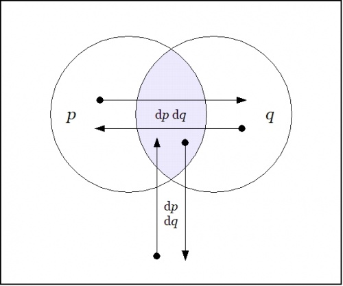
The field of changes produced by $\mathrm{D}\!$ on $pq\!$ is shown in the following venn diagram:

$\text{Difference}~ \mathrm{D}(pq) : \mathrm{E}X \to \mathbb{B}~\!$

$\begin{array}{rcccccc} \mathrm{D}(pq) & = & p & \cdot & q & \cdot & \texttt{(} \texttt{(} \mathrm{d}p \texttt{)} \texttt{(} \mathrm{d}q \texttt{)} \texttt{)} \\[4pt] & + & p & \cdot & \texttt{(} q \texttt{)} & \cdot & \texttt{~} \texttt{(} \mathrm{d}p \texttt{)} \texttt{~} \mathrm{d}q \texttt{~} \texttt{~} \\[4pt] & + & \texttt{(} p \texttt{)} & \cdot & q & \cdot & \texttt{~} \texttt{~} \mathrm{d}p \texttt{~} \texttt{(} \mathrm{d}q \texttt{)} \texttt{~} \\[4pt] & + & \texttt{(} p \texttt{)} & \cdot & \texttt{(}q \texttt{)} & \cdot & \texttt{~} \texttt{~} \mathrm{d}p \texttt{~} \texttt{~} \mathrm{d}q \texttt{~} \texttt{~} \end{array}\!$

The differential field $\mathrm{D}(pq)\!$ specifies the changes that need to be made from each point of $X\!$ in order to feel a change in the felt value of the field $pq.\!$

Proposition and Tacit Extension

Now that we've introduced the field picture as an aid to thinking about propositions and their analytic series, a very pleasing way of picturing the relationships among a proposition $f : X \to \mathbb{B},\!$ its enlargement or shift map $\mathrm{E}f : \mathrm{E}X \to \mathbb{B},\!$ and its difference map $\mathrm{D}f : \mathrm{E}X \to \mathbb{B}\!$ can now be drawn.

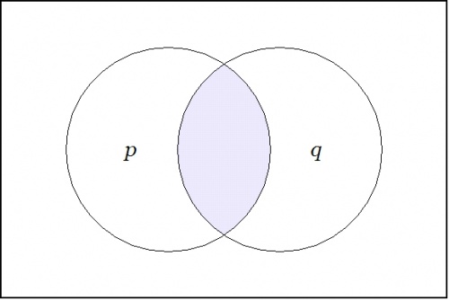
To illustrate this possibility, let's return to the differential analysis of the conjunctive proposition $f(p, q) = pq,\!$ giving the development a slightly different twist at the appropriate point.

The next venn diagram shows once again the proposition $pq,\!$ which we now view as a scalar field — analogous to a potential hill in physics, but in logic tantamount to a potential plateau — where the shaded region indicates an elevation of 1 and the unshaded region indicates an elevation of 0.

$\text{Proposition}~ pq : X \to \mathbb{B}\!$

Given a proposition $f : X \to \mathbb{B},\!$ the tacit extension of $f\!$ to $\mathrm{E}X\!$ is denoted $\boldsymbol\varepsilon f : \mathrm{E}X \to \mathbb{B}~\!$ and defined by the equation $\boldsymbol\varepsilon f = f,\!$ so it's really just the same proposition residing in a bigger universe. Tacit extensions formalize the intuitive idea that a function on a particular set of variables can be extended to a function on a superset of those variables in such a way that the new function obeys the same constraints on the old variables, with a "don't care" condition on the new variables.

The tacit extension of the scalar field $pq : X \to \mathbb{B}\!$ to the differential field $\boldsymbol\varepsilon (pq) : \mathrm{E}X \to \mathbb{B}\!$ is shown in the following venn diagram:

$\text{Tacit Extension}~ \boldsymbol\varepsilon (pq) : \mathrm{E}X \to \mathbb{B}~\!$

$\begin{array}{rcccccc} \boldsymbol\varepsilon (pq) & = & p & \cdot & q & \cdot & \texttt{(} \mathrm{d}p \texttt{)} \texttt{(} \mathrm{d}q \texttt{)} \\[4pt] & + & p & \cdot & q & \cdot & \texttt{(} \mathrm{d}p \texttt{)} \texttt{~} \mathrm{d}q \texttt{~} \\[4pt] & + & p & \cdot & q & \cdot & \texttt{~} \mathrm{d}p \texttt{~} \texttt{(} \mathrm{d}q \texttt{)} \\[4pt] & + & p & \cdot & q & \cdot & \texttt{~} \mathrm{d}p \texttt{~} \texttt{~} \mathrm{d}q \texttt{~} \end{array}\!$

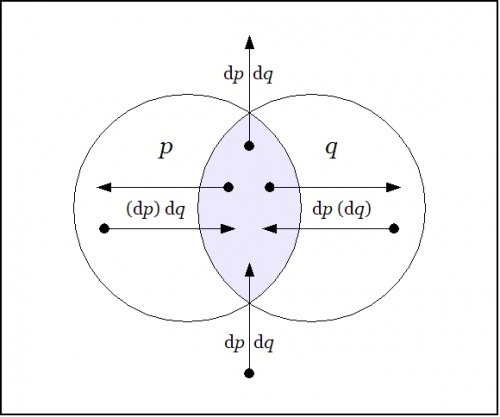
Enlargement and Difference Maps

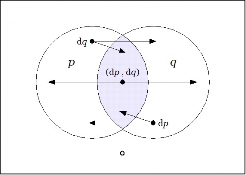
Continuing with the example $pq : X \to \mathbb{B},\!$ the next venn diagram shows the enlargement or shift map $\mathrm{E}(pq) : \mathrm{E}X \to \mathbb{B}\!$ in the same style of differential field picture that we drew for the tacit extension $\boldsymbol\varepsilon (pq) : \mathrm{E}X \to \mathbb{B}.\!$

$\text{Enlargement Map}~ \mathrm{E}(pq) : \mathrm{E}X \to \mathbb{B}\!$

$\begin{array}{rcccccc} \mathrm{E}(pq) & = & p & \cdot & q & \cdot & \texttt{(} \mathrm{d}p \texttt{)} \texttt{(} \mathrm{d}q \texttt{)} \\[4pt] & + & p & \cdot & \texttt{(} q \texttt{)} & \cdot & \texttt{(} \mathrm{d}p \texttt{)} \texttt{~} \mathrm{d}q \texttt{~} \\[4pt] & + & \texttt{(} p \texttt{)} & \cdot & q & \cdot & \texttt{~} \mathrm{d}p \texttt{~} \texttt{(} \mathrm{d}q \texttt{)} \\[4pt] & + & \texttt{(} p \texttt{)} & \cdot & \texttt{(} q \texttt{)} & \cdot & \texttt{~} \mathrm{d}p \texttt{~} \texttt{~} \mathrm{d}q \texttt{~} \end{array}\!$

A very important conceptual transition has just occurred here, almost tacitly, as it were. Generally speaking, having a set of mathematical objects of compatible types, in this case the two differential fields $\boldsymbol\varepsilon f\!$ and $\mathrm{E}f,\!$ both of the type $\mathrm{E}X \to \mathbb{B},\!$ is very useful, because it allows us to consider these fields as integral mathematical objects that can be operated on and combined in the ways that we usually associate with algebras.

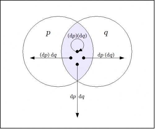
In this case one notices that the tacit extension $\boldsymbol\varepsilon f\!$ and the enlargement $\mathrm{E}f\!$ are in a certain sense dual to each other. The tacit extension $\boldsymbol\varepsilon f\!$ indicates all the arrows out of the region where $f\!$ is true and the enlargement $\mathrm{E}f\!$ indicates all the arrows into the region where $f\!$ is true. The only arc they have in common is the no-change loop $\texttt{(} \mathrm{d}p \texttt{)(} \mathrm{d}q \texttt{)}\!$ at $pq.\!$ If we add the two sets of arcs in mod 2 fashion then the loop of multiplicity 2 zeroes out, leaving the 6 arrows of $\mathrm{D}(pq) = \boldsymbol\varepsilon(pq) + \mathrm{E}(pq)\!$ that are illustrated below:

$\text{Difference Map}~ \mathrm{D}(pq) : \mathrm{E}X \to \mathbb{B}\!$

$\begin{array}{rcccccc} \mathrm{D}(pq) & = & p & \cdot & q & \cdot & \texttt{(} \texttt{(} \mathrm{d}p \texttt{)} \texttt{(} \mathrm{d}q \texttt{)} \texttt{)} \\[4pt] & + & p & \cdot & \texttt{(} q \texttt{)} & \cdot & \texttt{~} \texttt{(} \mathrm{d}p \texttt{)} \texttt{~} \mathrm{d}q \texttt{~} \texttt{~} \\[4pt] & + & \texttt{(} p \texttt{)} & \cdot & q & \cdot & \texttt{~} \texttt{~} \mathrm{d}p \texttt{~} \texttt{(} \mathrm{d}q \texttt{)} \texttt{~} \\[4pt] & + & \texttt{(} p \texttt{)} & \cdot & \texttt{(}q \texttt{)} & \cdot & \texttt{~} \texttt{~} \mathrm{d}p \texttt{~} \texttt{~} \mathrm{d}q \texttt{~} \texttt{~} \end{array}\!$

Tangent and Remainder Maps

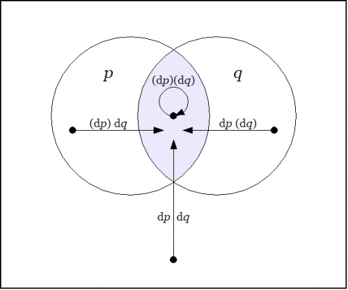
If we follow the classical line that singles out linear functions as ideals of simplicity, then we may complete the analytic series of the proposition $f = pq : X \to \mathbb{B}\!$ in the following way.

The next venn diagram shows the differential proposition $\mathrm{d}f = \mathrm{d}(pq) : \mathrm{E}X \to \mathbb{B}\!$ that we get by extracting the cell-wise linear approximation to the difference map $\mathrm{D}f = \mathrm{D}(pq) : \mathrm{E}X \to \mathbb{B}.\!$ This is the logical analogue of what would ordinarily be called the differential of $pq,\!$ but since I've been attaching the adjective differential to just about everything in sight, the distinction tends to be lost. For the time being, I'll resort to using the alternative name tangent map for $\mathrm{d}f.\!$

$\text{Tangent Map}~ \mathrm{d}(pq) : \mathrm{E}X \to \mathbb{B}\!$

Just to be clear about what's being indicated here, it's a visual way of summarizing the following data:

$\begin{array}{rcccccc} \mathrm{d}(pq) & = & p & \cdot & q & \cdot & \texttt{(} \mathrm{d}p \texttt{,} \mathrm{d}q \texttt{)} \\[4pt] & + & p & \cdot & \texttt{(} q \texttt{)} & \cdot & \mathrm{d}q \\[4pt] & + & \texttt{(} p \texttt{)} & \cdot & q & \cdot & \mathrm{d}p \\[4pt] & + & \texttt{(} p \texttt{)} & \cdot & \texttt{(} q \texttt{)} & \cdot & 0 \end{array}\!$

To understand the extended interpretations, that is, the conjunctions of basic and differential features that are being indicated here, it may help to note the following equivalences:

$\begin{matrix} \texttt{(} \mathrm{d}p \texttt{,} \mathrm{d}q \texttt{)} & = & \texttt{~} \mathrm{d}p \texttt{~} \texttt{(} \mathrm{d}q \texttt{)} & + & \texttt{(} \mathrm{d}p \texttt{)} \texttt{~} \mathrm{d}q \texttt{~} \\[4pt] dp & = & \texttt{~} \mathrm{d}p \texttt{~} \texttt{~} \mathrm{d}q \texttt{~} & + & \texttt{~} \mathrm{d}p \texttt{~} \texttt{(} \mathrm{d}q \texttt{)} \\[4pt] \mathrm{d}q & = & \texttt{~} \mathrm{d}p \texttt{~} \texttt{~} \mathrm{d}q \texttt{~} & + & \texttt{(} \mathrm{d}p \texttt{)} \texttt{~} \mathrm{d}q \texttt{~} \end{matrix}\!$

Capping the series that analyzes the proposition $pq\!$ in terms of succeeding orders of linear propositions, the final venn diagram in this series shows the remainder map $\mathrm{r}(pq) : \mathrm{E}X \to \mathbb{B},\!$ that happens to be linear in pairs of variables.

$\text{Remainder Map}~ \mathrm{r}(pq) : \mathrm{E}X \to \mathbb{B}\!$

Reading the arrows off the map produces the following data:

$\begin{array}{rcccccc} \mathrm{r}(pq) & = & p & \cdot & q & \cdot & \mathrm{d}p ~ \mathrm{d}q \\[4pt] & + & p & \cdot & \texttt{(} q \texttt{)} & \cdot & \mathrm{d}p ~ \mathrm{d}q \\[4pt] & + & \texttt{(} p \texttt{)} & \cdot & q & \cdot & \mathrm{d}p ~ \mathrm{d}q \\[4pt] & + & \texttt{(} p \texttt{)} & \cdot & \texttt{(} q \texttt{)} & \cdot & \mathrm{d}p ~ \mathrm{d}q \end{array}\!$

In short, $\mathrm{r}(pq)\!$ is a constant field, having the value $\mathrm{d}p~\mathrm{d}q\!$ at each cell.

Least Action Operators

We have been contemplating functions of the type $f : X \to \mathbb{B}\!$ and studying the action of the operators $\mathrm{E}\!$ and $\mathrm{D}\!$ on this family. These functions, that we may identify for our present aims with propositions, inasmuch as they capture their abstract forms, are logical analogues of scalar potential fields. These are the sorts of fields that are so picturesquely presented in elementary calculus and physics textbooks by images of snow-covered hills and parties of skiers who trek down their slopes like least action heroes. The analogous scene in propositional logic presents us with forms more reminiscent of plateaunic idylls, being all plains at one of two levels, the mesas of verity and falsity, as it were, with nary a niche to inhabit between them, restricting our options for a sporting gradient of downhill dynamics to just one of two: standing still on level ground or falling off a bluff.

We are still working well within the logical analogue of the classical finite difference calculus, taking in the novelties that the logical transmutation of familiar elements is able to bring to light. Soon we will take up several different notions of approximation relationships that may be seen to organize the space of propositions, and these will allow us to define several different forms of differential analysis applying to propositions. In time we will find reason to consider more general types of maps, having concrete types of the form $X_1 \times \ldots \times X_k \to Y_1 \times \ldots \times Y_n\!$ and abstract types $\mathbb{B}^k \to \mathbb{B}^n.\!$ We will think of these mappings as transforming universes of discourse into themselves or into others, in short, as transformations of discourse.

Before we continue with this intinerary, however, I would like to highlight another sort of differential aspect that concerns the boundary operator or the marked connective that serves as one of the two basic connectives in the cactus language for zeroth order logic.

For example, consider the proposition $f\!$ of concrete type $f : P \times Q \times R \to \mathbb{B}\!$ and abstract type $f : \mathbb{B}^3 \to \mathbb{B}\!$ that is written $\texttt{(} p, q, r \texttt{)}\!$ in cactus syntax. Taken as an assertion in what Peirce called the existential interpretation, the proposition $\texttt{(} p, q, r \texttt{)}\!$ says that just one of $p, q, r\!$ is false. It is instructive to consider this assertion in relation to the logical conjunction $pqr\!$ of the same propositions. A venn diagram of $\texttt{(} p, q, r \texttt{)}\!$ looks like this:

In relation to the center cell indicated by the conjunction $pqr,\!$ the region indicated by $\texttt{(} p, q, r \texttt{)}\!$ is comprised of the adjacent or bordering cells. Thus they are the cells that are just across the boundary of the center cell, reached as if by way of Leibniz's minimal changes from the point of origin, in this case, $pqr.~\!$

More generally speaking, in a $k\!$ -dimensional universe of discourse that is based on the alphabet of features $\mathcal{X} = \{ x_1, \ldots, x_k \},\!$ the same form of boundary relationship is manifested for any cell of origin that one chooses to indicate. One way to indicate a cell is by forming a logical conjunction of positive and negative basis features, that is, by constructing an expression of the form $e_1 \cdot \ldots \cdot e_k,\!$ where $e_j = x_j ~\text{or}~ e_j = \texttt{(} x_j \texttt{)},\!$ for $j = 1 ~\text{to}~ k.\!$ The proposition $\texttt{(} e_1, \ldots, e_k \texttt{)}\!$ indicates the disjunctive region consisting of the cells that are just next door to $e_1 \cdot \ldots \cdot e_k.\!$

Goal-Oriented Systems

I want to continue developing the basic tools of differential logic, which arose from exploring the connections between dynamics and logic, but I also wanted to give some hint of the applications that have motivated this work all along. One of these applications is to cybernetic systems, whether we see these systems as agents or cultures, individuals or species, organisms or organizations.

A cybernetic system has goals and actions for reaching them. It has a state space $X,\!$ giving us all of the states that the system can be in, plus it has a goal space $G \subseteq X,\!$ the set of states that the system “likes” to be in, in other words, the distinguished subset of possible states where the system is regarded as living, surviving, or thriving, depending on the type of goal that one has in mind for the system in question. As for actions, there is to begin with the full set $\mathcal{T}\!$ of all possible actions, each of which is a transformation of the form $T : X \to X,\!$ but a given cybernetic system will most likely have but a subset of these actions available to it at any given time. And even if we begin by thinking of actions in very general and very global terms, as arbitrarily complex transformations acting on the whole state space $X,\!$ we quickly find a need to analyze and approximate them in terms of simple transformations acting locally. The preferred measure of “simplicity” will of course vary from one paradigm of research to another.

A generic enough picture at this stage of the game, and one that will remind us of these fundamental features of the cybernetic system even as things get far more complex, is afforded by Figure 23.

o---------------------------------------------------------------------o
|                                                                     |
|   X                                                                 |
|            o-------------------o                                    |
|           /                     \                                   |
|          /                       \                                  |
|         /                         \                                 |
|        /                           \                                |
|       /                             \                               |
|      /                               \                              |
|     /                                 \                             |
|    o                 G                 o                            |
|    |                                   |                            |
|    |                                   |                            |
|    |                                   |                            |
|    |                        o<---------T---------o                  |
|    |                                   |                            |
|    |                                   |                            |
|    |                                   |                            |
|    o                                   o                            |
|     \                                 /                             |
|      \                               /                              |
|       \                             /                               |
|        \                           /                                |
|         \                         /                                 |
|          \                       /                                  |
|           \                     /                                   |
|            o-------------------o                                    |
|                                                                     |
|                                                                     |
o---------------------------------------------------------------------o
Figure 23.  Elements of a Cybernetic System

Document History

Differential Logic • Ontology List 2002

http://web.archive.org/web/20110612002240/http://suo.ieee.org/ontology/thrd28.html#04040

Dynamics And Logic • Inquiry List 2004

Dynamics And Logic • NKS Forum 2004

@@ Line 34: / Line 34: @@
 Table&nbsp;1 collects a sample of basic propositional forms as expressed in terms of cactus language connectives.
-{| align="center" border="1" cellpadding="8" cellspacing="0" style="text-align:center; width:90%"
+<br>
-|+ <math>\text{Table 1.}~~\text{Syntax and Semantics of a Calculus for Propositional Logic}\!</math>
-|- style="background:#f0f0ff"
+{| align="center" border="1" cellpadding="8" cellspacing="0" style="text-align:center; width:75%"
-| <math>\text{Graph}\!</math>
+|+ style="height:30px" | <math>\text{Table 1.} ~~ \text{Syntax and Semantics of a Calculus for Propositional Logic}\!</math>
+|- style="height:40px; background:ghostwhite"
 | <math>\text{Expression}~\!</math>
 | <math>\text{Interpretation}\!</math>
 | <math>\text{Other Notations}\!</math>
 |-
-| height="100px" | [[Image:Rooted Node.jpg|20px]]
+| &nbsp;
-| <math>~\!</math>
+| <math>\text{True}\!</math>
-| <math>\mathrm{true}\!</math>
 | <math>1\!</math>
 |-
-| height="100px" | [[Image:Rooted Edge.jpg|20px]]
 | <math>\texttt{(~)}\!</math>
-| <math>\mathrm{false}\!</math>
+| <math>\text{False}\!</math>
 | <math>0\!</math>
 |-
-| height="100px" | [[Image:Cactus A Big.jpg|20px]]
+| <math>x\!</math>
-| <math>a\!</math>
+| <math>x\!</math>
-| <math>a\!</math>
+| <math>x\!</math>
-| <math>a\!</math>
 |-
-| height="120px" | [[Image:Cactus (A) Big.jpg|20px]]
+| <math>\texttt{(} x \texttt{)}\!</math>
-| <math>\texttt{(} a \texttt{)}\!</math>
+| <math>\text{Not}~ x\!</math>
-| <math>\mathrm{not}~ a\!</math>
+|
-| <math>\lnot a \quad \bar{a} \quad \tilde{a} \quad a^\prime~\!</math>
+<math>\begin{matrix}
+x'
+\\
+\tilde{x}
+\\
+\lnot x
+\end{matrix}\!</math>
 |-
-| height="100px" | [[Image:Cactus ABC Big.jpg|50px]]
+| <math>x~y~z\!</math>
-| <math>a ~ b ~ c\!</math>
+| <math>x ~\text{and}~ y ~\text{and}~ z\!</math>
-| <math>a ~\mathrm{and}~ b ~\mathrm{and}~ c\!</math>
+| <math>x \land y \land z\!</math>
-| <math>a \land b \land c\!</math>
 |-
-| height="160px" | [[Image:Cactus ((A)(B)(C)) Big.jpg|65px]]
+| <math>\texttt{((} x \texttt{)(} y \texttt{)(} z \texttt{))}\!</math>
-| <math>\texttt{((} a \texttt{)(} b \texttt{)(} c \texttt{))}\!</math>
+| <math>x ~\text{or}~ y ~\text{or}~ z\!</math>
-| <math>a ~\mathrm{or}~ b ~\mathrm{or}~ c\!</math>
+| <math>x \lor y \lor z\!</math>
-| <math>a \lor b \lor c\!</math>
 |-
-| height="120px" | [[Image:Cactus (A(B)) Big.jpg|60px]]
+| <math>\texttt{(} x ~ \texttt{(} y \texttt{))}\!</math>
-| <math>\texttt{(} a \texttt{(} b \texttt{))}\!</math>
 |
 <math>\begin{matrix}
-a ~\text{implies}~ b
+x ~\text{implies}~ y
-\\[6pt]
+\\
-\mathrm{if}~ a ~\mathrm{then}~ b
+\mathrm{If}~ x ~\text{then}~ y
-\end{matrix}\!</math>
+\end{matrix}</math>
-| <math>a \Rightarrow b\!</math>
+| <math>x \Rightarrow y\!</math>
 |-
-| height="120px" | [[Image:Cactus (A,B) Big ISW.jpg|65px]]
+| <math>\texttt{(} x \texttt{,} y \texttt{)}\!</math>
-| <math>\texttt{(} a \texttt{,} b \texttt{)}\!</math>
 |
 <math>\begin{matrix}
-a ~\mathrm{not~equal~to}~ b
+x ~\text{not equal to}~ y
-\\[6pt]
+\\
-a ~\mathrm{exclusive~or}~ b
+x ~\text{exclusive or}~ y
-\end{matrix}\!</math>
+\end{matrix}</math>
 |
 <math>\begin{matrix}
-a \neq b
+x \ne y
-\\[6pt]
+\\
-a + b
+x + y
-\end{matrix}\!</math>
+\end{matrix}</math>
 |-
-| height="160px" | [[Image:Cactus ((A,B)) Big.jpg|65px]]
+| <math>\texttt{((} x \texttt{,} y \texttt{))}\!</math>
-| <math>\texttt{((} a \texttt{,} b \texttt{))}\!</math>
 |
 <math>\begin{matrix}
-a ~\mathrm{is~equal~to}~ b
+x ~\text{is equal to}~ y
-\\[6pt]
+\\
-a ~\mathrm{if~and~only~if}~ b
+x ~\text{if and only if}~ y
-\end{matrix}\!</math>
+\end{matrix}</math>
 |
 <math>\begin{matrix}
-a = b
+x = y
-\\[6pt]
+\\
-a \Leftrightarrow b
+x \Leftrightarrow y
-\end{matrix}\!</math>
+\end{matrix}</math>
 |-
-| height="120px" | [[Image:Cactus (A,B,C) Big.jpg|65px]]
+| <math>\texttt{(} x \texttt{,} y \texttt{,} z \texttt{)}\!</math>
-| <math>\texttt{(} a \texttt{,} b \texttt{,} c \texttt{)}\!</math>
 |
 <math>\begin{matrix}
-\mathrm{just~one~of}
+\text{Just one of}
 \\
-a, b, c
+x, y, z
 \\
-\mathrm{is~false}.
+\text{is false}.
-\end{matrix}\!</math>
+\end{matrix}</math>
 |
 <math>\begin{matrix}
-& \bar{a} ~ b ~ c
+x'y~z~ & \lor
 \\
-\lor & a ~ \bar{b} ~ c
+x~y'z~ & \lor
 \\
-\lor & a ~ b ~ \bar{c}
+x~y~z' &
-\end{matrix}\!</math>
+\end{matrix}</math>
 |-
-| height="160px" | [[Image:Cactus ((A),(B),(C)) Big.jpg|65px]]
+| <math>\texttt{((} x \texttt{),(} y \texttt{),(} z \texttt{))}\!</math>
-| <math>\texttt{((} a \texttt{),(} b \texttt{),(} c \texttt{))}\!</math>
 |
 <math>\begin{matrix}
-\mathrm{just~one~of}
+\text{Just one of}
+\\
+x, y, z
+\\
+\text{is true}.
+\\
+&
+\\
+\text{Partition all}
 \\
-a, b, c
+\text{into}~ x, y, z.
+\end{matrix}</math>
+|
+<math>\begin{matrix}
+x~y'z' & \lor
 \\
-\mathrm{is~true}.
+x'y~z' & \lor
-\\[6pt]
-\mathrm{partition~all}
 \\
-\mathrm{into}~ a, b, c.
+x'y'z~ &
-\end{matrix}\!</math>
+\end{matrix}</math>
+|-
 |
 <math>\begin{matrix}
-& a ~ \bar{b} ~ \bar{c}
+\texttt{((} x \texttt{,} y \texttt{),} z \texttt{)}
 \\
-\lor & \bar{a} ~ b ~ \bar{c}
+&
 \\
-\lor & \bar{a} ~ \bar{b} ~ c
+\texttt{(} x \texttt{,(} y \texttt{,} z \texttt{))}
 \end{matrix}\!</math>
-|-
-| height="160px" | [[Image:Cactus (A,(B,C)) Big.jpg|90px]]
-| <math>\texttt{(} a \texttt{,(} b \texttt{,} c \texttt{))}\!</math>
 |
 <math>\begin{matrix}
-\mathrm{oddly~many~of}
+\text{Oddly many of}
 \\
-a, b, c
+x, y, z
 \\
-\mathrm{are~true}.
+\text{are true}.
 \end{matrix}\!</math>
 |
-<p><math>a + b + c\!</math></p>
+<p><math>x + y + z\!</math></p>
 <br>
 <p><math>\begin{matrix}
-& a ~ b ~ c
+x~y~z~ & \lor
 \\
-\lor & a ~ \bar{b} ~ \bar{c}
+x~y'z' & \lor
 \\
-\lor & \bar{a} ~ b ~ \bar{c}
+x'y~z' & \lor
 \\
-\lor & \bar{a} ~ \bar{b} ~ c
+x'y'z~ &
 \end{matrix}\!</math></p>
 |-
-| height="160px" | [[Image:Cactus (X,(A),(B),(C)) Big.jpg|90px]]
+| <math>\texttt{(} w \texttt{,(} x \texttt{),(} y \texttt{),(} z \texttt{))}\!</math>
-| <math>\texttt{(} x \texttt{,(} a \texttt{),(} b \texttt{),(} c \texttt{))}\!</math>
 |
 <math>\begin{matrix}
-\mathrm{partition}~ x
+\text{Partition}~ w
 \\
-\mathrm{into}~ a, b, c.
+\text{into}~ x, y, z.
-\\[6pt]
-\mathrm{genus}~ x ~\mathrm{comprises}
 \\
-\mathrm{species}~ a, b, c.
+&
-\end{matrix}\!</math>
+\\
+\text{Genus}~ w ~\text{comprises}
+\\
+\text{species}~ x, y, z.
+\end{matrix}</math>
 |
 <math>\begin{matrix}
-& \bar{x} ~ \bar{a} ~ \bar{b} ~ \bar{c}
+w'x'y'z' & \lor
 \\
-\lor & x ~ a ~ \bar{b} ~ \bar{c}
+w~x~y'z' & \lor
 \\
-\lor & x ~ \bar{a} ~ b ~ \bar{c}
+w~x'y~z' & \lor
 \\
-\lor & x ~ \bar{a} ~ \bar{b} ~ c
+w~x'y'z~ &
-\end{matrix}~\!</math>
+\end{matrix}</math>
 |}
+<br>
 The simplest expression for logical truth is the empty word, usually denoted by <math>\boldsymbol\varepsilon\!</math> or <math>\lambda\!</math> in formal languages, where it forms the identity element for concatenation.  To make it visible in context, it may be denoted by the equivalent expression <math>{}^{\backprime\backprime} \texttt{((~))} {}^{\prime\prime},\!</math> or, especially if operating in an algebraic context, by a simple <math>{}^{\backprime\backprime} 1 {}^{\prime\prime}.\!</math>  Also when working in an algebraic mode, the plus sign <math>{}^{\backprime\backprime} + {}^{\prime\prime}\!</math> may be used for [[exclusive disjunction]].  For example, we have the following paraphrases of algebraic expressions by means of parenthesized expressions:

Difference between revisions of "Directory:Jon Awbrey/Papers/Differential Logic : Introduction"

Revision as of 16:38, 29 November 2015

Contents

Quick Overview

Cactus Language for Propositional Logic

Differential Expansions of Propositions

Bird's Eye View

Worm's Eye View

Quick Review : Field Picture

Proposition and Tacit Extension

Enlargement and Difference Maps

Tangent and Remainder Maps

Least Action Operators

Goal-Oriented Systems

Further Reading

Document History

Differential Logic • Ontology List 2002

Dynamics And Logic • Inquiry List 2004

Dynamics And Logic • NKS Forum 2004

Navigation menu

Page actions

Page actions

Personal tools

Navigation

semantic

Site statistics

Tools

Search