Differential Propositional Calculus

A differential propositional calculus is a propositional calculus extended by a set of terms for describing aspects of change and difference, for example, processes that take place in a universe of discourse or transformations that map a source universe into a target universe.

1. Casual Introduction

Consider the situation represented by the venn diagram in Figure 1.

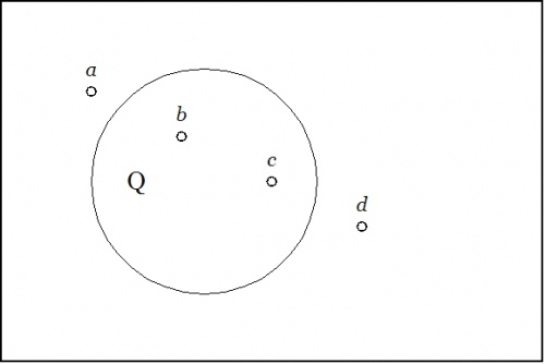
Figure 1. Local Habitations, And Names

The area of the rectangle represents a universe of discourse, $X.\!$ This might be a population of individuals having various additional properties or it might be a collection of locations that various individuals occupy. The area of the "circle" represents the individuals that have the property $q\!$ or the locations that fall within the corresponding region $Q.\!$ Four individuals, $a, b, c, d,\!$ are singled out by name. It happens that $b\!$ and $c\!$ currently reside in region $Q\!$ while $a\!$ and $d\!$ do not.

Now consider the situation represented by the venn diagram in Figure 2.

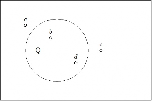
Figure 2. Same Names, Different Habitations

Figure 2 differs from Figure 1 solely in the circumstance that the object $c\!$ is outside the region $Q\!$ while the object $d\!$ is inside the region $Q.\!$ So far, there is nothing that says that our encountering these Figures in this order is other than purely accidental, but if we interpret the present sequence of frames as a "moving picture" representation of their natural order in a temporal process, then it would be natural to say that $a\!$ and $b\!$ have remained as they were with regard to quality $q\!$ while $c\!$ and $d\!$ have changed their standings in that respect. In particular, $c\!$ has moved from the region where $q\!$ is $true\!$ to the region where $q\!$ is $false\!$ while $d\!$ has moved from the region where $q\!$ is $false\!$ to the region where $q\!$ is $true.\!$

Figure 1′ reprises the situation shown in Figure 1, but this time interpolates a new quality that is specifically tailored to account for the relation between Figure 1 and Figure 2.

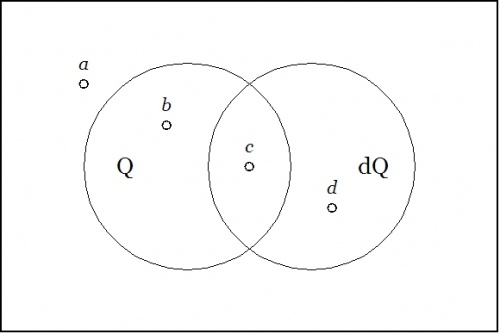
Figure 1′. Back, To The Future

This new quality, $\operatorname{d}q,\!$ is an example of a differential quality, since its absence or presence qualifies the absence or presence of change occurring in another quality. As with any other quality, it is represented in the venn diagram by means of a "circle" that distinguishes two halves of the universe of discourse, in this case, the portions of $X\!$ outside and inside the region $\operatorname{d}Q.\!$

Figure 1 represents a universe of discourse, $X,\!$ together with a basis of discussion, $\{ q \},\!$ for expressing propositions about the contents of that universe. Once the quality $q\!$ is given a name, say, the symbol "$q\!$", we have the basis for a formal language that is specifically cut out for discussing $X\!$ in terms of $q,\!$ and this formal language is more formally known as the propositional calculus with alphabet $\{\!$"$q\!$"$\}.\!$

In the context marked by $X\!$ and $\{ q \}\!$ there are but four different pieces of information that can be expressed in the corresponding propositional calculus, namely, the propositions $$false,\!$$ $\lnot q,\!$ $q,\!$ $true.\!$ Referring to the sample of points in Figure 1, $false\!$ holds of no points, $\lnot q\!$ holds of $a\!$ and $d,\!$ $q\!$ holds of $b\!$ and $c,\!$ and $true\!$ holds of all points in the sample.

Figure 1′ preserves the same universe of discourse and extends the basis of discussion to a set of two qualities, $\{ q, \operatorname{d}q \}.\!$ In parallel fashion, the initial propositional calculus is extended by means of the enlarged alphabet, $\{\!$"$q\!$"$,\!$ "$\operatorname{d}q\!$"$\}.\!$ Any propositional calculus over two basic propositions allows for the expression of 16 propositions all together. Just by way of salient examples in the present setting, we can pick out the most informative propositions that apply to each of our sample points. Using overlines to express logical negation, these are given as follows:

• $\overline{q}\ \overline{\operatorname{d}q}$ describes $a\!$

• $\overline{q}\ \operatorname{d}q$ describes $d\!$

• $q\ \overline{\operatorname{d}q}$ describes $b\!$

• $q\ \operatorname{d}q$ describes $c\!$

Table 3 exhibits the rules of inference that give the differential quality $\operatorname{d}q\!$ its meaning in practice.

Table 3. Differential Inference Rules

From $\overline{q}\!$ and $\overline{\operatorname{d}q}\!$ infer $\overline{q}\!$ next.     From $\overline{q}\!$ and $\operatorname{d}q\!$ infer $q\!$ next.     From $q\!$ and $\overline{\operatorname{d}q}\!$ infer $q\!$ next.     From $q\!$ and $\operatorname{d}q\!$ infer $\overline{q}\!$ next.

2. Cactus Calculus

Table 4 outlines a syntax for propositional calculus based on two types of logical connectives, both of variable $k\!$-ary scope.

• A bracketed list of propositional expressions in the form $(e_1, e_2, \ldots, e_{k-1}, e_k)$ indicates that exactly one of the propositions $e_1, e_2, \ldots, e_{k-1}, e_k$ is false.

• A concatenation of propositional expressions in the form $e_1~e_2~\ldots~e_{k-1}~e_k$ indicates that all of the propositions $e_1, e_2, \ldots, e_{k-1}, e_k$ are true, in other words, that their logical conjunction is true.

Table 4. Syntax and Semantics of a Propositional Calculus

Expression	Interpretation	Other Notations
$~$	$\operatorname{True}$	$1\!$
$(~)$	$\operatorname{False}$	$0\!$
$x\!$	$x\!$	$x\!$
$(x)\!$	$\operatorname{Not}\ x$	$\begin{matrix} x' \\ \tilde{x} \\ \lnot x \\ \end{matrix}$
$x\ y\ z$	$x\ \operatorname{and}\ y\ \operatorname{and}\ z$	$x \land y \land z$
$((x)(y)(z))\!$	$x\ \operatorname{or}\ y\ \operatorname{or}\ z$	$x \lor y \lor z$
$(x\ (y))\!$	$\begin{matrix} x\ \operatorname{implies}\ y \\ \operatorname{If}\ x\ \operatorname{then}\ y \\ \end{matrix}$	$x \Rightarrow y\!$
$(x, y)\!$	$\begin{matrix} x\ \operatorname{not~equal~to}\ y \\ x\ \operatorname{exclusive~or}\ y \\ \end{matrix}$	$\begin{matrix} x \neq y \\ x + y \\ \end{matrix}$
$((x, y))\!$	$\begin{matrix} x\ \operatorname{is~equal~to}\ y \\ x\ \operatorname{if~and~only~if}\ y \\ \end{matrix}$	$\begin{matrix} x = y \\ x \Leftrightarrow y \\ \end{matrix}$
$(x, y, z)\!$	$\begin{matrix} \operatorname{Just~one~of} \\ x, y, z \\ \operatorname{is~false}. \\ \end{matrix}$	$\begin{matrix} x'y~z~ & \lor \\ x~y'z~ & \lor \\ x~y~z' & \\ \end{matrix}$
$((x),(y),(z))\!$	$\begin{matrix} \operatorname{Just~one~of} \\ x, y, z \\ \operatorname{is~true}. \\ & \\ \operatorname{Partition~all} \\ \operatorname{into}\ x, y, z. \\ \end{matrix}$	$\begin{matrix} x~y'z' & \lor \\ x'y~z' & \lor \\ x'y'z~ & \\ \end{matrix}$
$\begin{matrix} ((x, y), z) \\ & \\ (x, (y, z)) \\ \end{matrix}$	$\begin{matrix} \operatorname{Oddly~many~of} \\ x, y, z \\ \operatorname{are~true}. \\ \end{matrix}$	$x + y + z\!$ $\begin{matrix} x~y~z~ & \lor \\ x~y'z' & \lor \\ x'y~z' & \lor \\ x'y'z~ & \\ \end{matrix}$
$(w, (x),(y),(z))\!$	$\begin{matrix} \operatorname{Partition}\ w \\ \operatorname{into}\ x, y, z. \\ & \\ \operatorname{Genus}\ w\ \operatorname{comprises} \\ \operatorname{species}\ x, y, z. \\ \end{matrix}$	$\begin{matrix} w'x'y'z' & \lor \\ w~x~y'z' & \lor \\ w~x'y~z' & \lor \\ w~x'y'z~ & \\ \end{matrix}$

All other propositional connectives can be obtained through combinations of these two forms. Strictly speaking, the concatenation form is dispensable in light of the bracket form, but it is convenient to maintain it as an abbreviation for more complicated bracket expressions. The briefest expression for logical truth is the empty word, abstractly denoted $\varepsilon\!$ or $\lambda\!$ in formal languages, where it forms the identity element for concatenation. It can be given visible expression in this context by means of the logically equivalent expression "$((~))$", or, especially if operating in an algebraic context, by a simple "$1\!$". Also when working in an algebraic mode, the plus sign "$+\!$ may be used for exclusive disjunction. For example, we have the following paraphrases of algebraic expressions by bracket expressions:

$\begin{matrix} x + y & = & (x, y) \end{matrix}$

$\begin{matrix} x + y + z & = & ((x, y), z) & = & (x, (y, z)) \end{matrix}$

It is important to note that the last expressions are not equivalent to the triple bracket $(x, y, z).\!$

For more information about this syntax for propositional calculus, see the entries on minimal negation operators, zeroth order logic, and Table A1 in Appendix 1.

3. Formal Development

The preceding discussion outlined the ideas leading to the differential extension of propositional logic. The next task is to lay out the concepts and terminology that are needed to describe various orders of differential propositional calculi.

3.1. Elementary Notions

Logical description of a universe of discourse begins with a set of logical signs. For the sake of simplicity in a first approach, assume that these logical signs are collected in the form of a finite alphabet, $\mathfrak{A} = \lbrace\!$ “$a_1\!$” $, \ldots,\!$ “$a_n\!$” $\rbrace.\!$ Each of these signs is interpreted as denoting a logical feature, for instance, a property that objects in the universe of discourse may have or a proposition about objects in the universe of discourse. Corresponding to the alphabet $\mathfrak{A}$ there is then a set of logical features, $\mathcal{A} = \{ a_1, \ldots, a_n \}.$

A set of logical features, $\mathcal{A} = \{ a_1, \ldots, a_n \},$ affords a basis for generating an $n\!$-dimensional universe of discourse, written $A^\circ = [ \mathcal{A} ] = [ a_1, \ldots, a_n ].$ It is useful to consider a universe of discourse as a categorical object that incorporates both the set of points $A = \langle a_1, \ldots, a_n \rangle$ and the set of propositions $A^\uparrow = \{ f : A \to \mathbb{B} \}$ that are implicit with the ordinary picture of a venn diagram on $n\!$ features. Accordingly, the universe of discourse $A^\circ$ may be regarded as an ordered pair $(A, A^\uparrow)$ having the type $(\mathbb{B}^n, (\mathbb{B}^n \to \mathbb{B})),$ and this last type designation may be abbreviated as $\mathbb{B}^n\ +\!\to \mathbb{B},$ or even more succinctly as $[ \mathbb{B}^n ].$ For convenience, the data type of a finite set on $n\!$ elements may be indicated by either one of the equivalent notations, $[n]\!$ or $\mathbf{n}.$

Table 5 summarizes the notations that are needed to describe ordinary propositional calculi in a systematic fashion.

Table 5. Propositional Calculus : Basic Notation

Symbol	Notation	Description	Type
$\mathfrak{A}$	$\lbrace\!$ “$a_1\!$” $, \ldots,\!$ “$a_n\!$” $\rbrace\!$	Alphabet	$[n] = \mathbf{n}$
$\mathcal{A}$	$\{ a_1, \ldots, a_n \}$	Basis	$[n] = \mathbf{n}$
$A_i\!$	$\{ \overline{a_i}, a_i \}\!$	Dimension $i\!$	$\mathbb{B}$
$A\!$	$\langle \mathcal{A} \rangle$ $\langle a_1, \ldots, a_n \rangle$ $\{ (a_1, \ldots, a_n) \}\!$ $A_1 \times \ldots \times A_n$ $\textstyle \prod_i A_i\!$	Set of cells, coordinate tuples, points, or vectors in the universe of discourse	$\mathbb{B}^n$
$A^*\!$	$(\operatorname{hom} : A \to \mathbb{B})$	Linear functions	$(\mathbb{B}^n)^* \cong \mathbb{B}^n$
$A^\uparrow$	$(A \to \mathbb{B})$	Boolean functions	$\mathbb{B}^n \to \mathbb{B}$
$A^\circ$	$[ \mathcal{A} ]$ $(A, A^\uparrow)$ $(A\ +\!\to \mathbb{B})$ $(A, (A \to \mathbb{B}))$ $[ a_1, \ldots, a_n ]$	Universe of discourse based on the features $\{ a_1, \ldots, a_n \}$	$(\mathbb{B}^n, (\mathbb{B}^n \to \mathbb{B}))$ $(\mathbb{B}^n\ +\!\to \mathbb{B})$ $[\mathbb{B}^n]$

3.2. Special Classes of Propositions

A basic proposition, coordinate proposition, or simple proposition in the universe of discourse $[a_1, \ldots, a_n]$ is one of the propositions in the set $\{ a_1, \ldots, a_n \}.$

Among the $2^{2^n}$ propositions in $[a_1, \ldots, a_n]$ are several families of $2^n\!$ propositions each that take on special forms with respect to the basis $\{ a_1, \ldots, a_n \}.$ Three of these families are especially prominent in the present context, the linear, the positive, and the singular propositions. Each family is naturally parameterized by the coordinate $n\!$-tuples in $\mathbb{B}^n$ and falls into $n + 1\!$ ranks, with a binomial coefficient $\tbinom{n}{k}$ giving the number of propositions that have rank or weight $k.\!$

• The linear propositions, $\{ \ell : \mathbb{B}^n \to \mathbb{B} \} = (\mathbb{B}^n \xrightarrow{\ell} \mathbb{B}),$ may be written as sums:

  $\sum_{i=1}^n e_i = e_1 + \ldots + e_n$  where  $e_i = a_i\!$  or  $e_i = 0\!$  for  $i = 1\!$  to  $n.\!$

• The positive propositions, $\{ p : \mathbb{B}^n \to \mathbb{B} \} = (\mathbb{B}^n \xrightarrow{p} \mathbb{B}),$ may be written as products:

  $\prod_{i=1}^n e_i = e_1 \cdot \ldots \cdot e_n$  where  $e_i = a_i\!$  or  $e_i = 1\!$  for  $i = 1\!$  to  $n.\!$

• The singular propositions, $\{ \mathbf{x} : \mathbb{B}^n \to \mathbb{B} \} = (\mathbb{B}^n \xrightarrow{s} \mathbb{B}),$ may be written as products:

  $\prod_{i=1}^n e_i = e_1 \cdot \ldots \cdot e_n$  where  $e_i = a_i\!$  or  $e_i = (a_i)\!$  for  $i = 1\!$  to  $n.\!$

In each case the rank $k\!$ ranges from $0\!$ to $n\!$ and counts the number of positive appearances of the coordinate propositions $a_1, \ldots, a_n\!$ in the resulting expression. For example, for $n = 3,\!$ the linear proposition of rank $0\!$ is $0,\!$ the positive proposition of rank $0\!$ is $1,\!$ and the singular proposition of rank $0\!$ is $(a_1)(a_2)(a_3).\!$

The basic propositions $a_i : \mathbb{B}^n \to \mathbb{B}$ are both linear and positive. So these two kinds of propositions, the linear and the positive, may be viewed as two different ways of generalizing the class of basic propositions.

Finally, it is important to note that all of the above distinctions are relative to the choice of a particular logical basis $\mathcal{A} = \{ a_1, \ldots, a_n \}.$ For example, a singular proposition with respect to the basis $\mathcal{A}$ will not remain singular if $\mathcal{A}$ is extended by a number of new and independent features. Even if one keeps to the original set of pairwise options $\{ a_i \} \cup \{ (a_i) \}$ to pick out a new basis, the sets of linear propositions and positive propositions are both determined by the choice of basic propositions, and this whole determination is tantamount to the purely conventional choice of a cell as origin.

3.3. Differential Extensions

An initial universe of discourse, $A^\circ,$ supplies the groundwork for any number of further extensions, beginning with the first order differential extension, $\operatorname{E}A^\circ.$ The construction of $\operatorname{E}A^\circ$ can be described in the following stages:

• The initial alphabet, $\mathfrak{A} = \lbrace\!$ “$a_1\!$” $, \ldots,\!$ “$a_n\!$” $\rbrace,\!$ is extended by a first order differential alphabet, $\operatorname{d}\mathfrak{A} = \lbrace\!$ “$\operatorname{d}a_1\!$” $, \ldots,\!$ “$\operatorname{d}a_n\!$” $\rbrace,\!$ resulting in a first order extended alphabet, $\operatorname{E}\mathfrak{A},$ defined as follows:

  $\operatorname{E}\mathfrak{A} = \mathfrak{A}\ \cup\ \operatorname{d}\mathfrak{A} = \lbrace\!$ “$a_1\!$” $, \ldots,\!$ “$a_n\!$”$,\!$  “$\operatorname{d}a_1\!$” $, \ldots,\!$ “$\operatorname{d}a_n\!$” $\rbrace.\!$

• The initial basis, $\mathcal{A} = \{ a_1, \ldots, a_n \},$ is extended by a first order differential basis, $\operatorname{d}\mathcal{A} = \{ \operatorname{d}a_1, \ldots, \operatorname{d}a_n \},$ resulting in a first order extended basis, $\operatorname{E}\mathcal{A},$ defined as follows:

  $\operatorname{E}\mathcal{A} = \mathcal{A}\ \cup\ \operatorname{d}\mathcal{A} = \{ a_1, \ldots, a_n, \operatorname{d}a_1, \ldots, \operatorname{d}a_n \}.$

• The initial space, $A = \langle a_1, \ldots, a_n \rangle,$ is extended by a first order differential space or tangent space, $\operatorname{d}A = \langle \operatorname{d}a_1, \ldots, \operatorname{d}a_n \rangle,$ at each point of $A,\!$ resulting in a first order extended space or tangent bundle space, $\operatorname{E}A,$ defined as follows:

  $\operatorname{E}A = A \times \operatorname{d}A = \langle \operatorname{E}\mathcal{A} \rangle = \langle \mathcal{A} \cup \operatorname{d}\mathcal{A} \rangle = \langle a_1, \ldots, a_n, \operatorname{d}a_1, \ldots, \operatorname{d}a_n \rangle.$

• Finally, the initial universe, $A^\circ = [ a_1, \ldots, a_n ],$ is extended by a first order differential universe or tangent universe, $\operatorname{d}A^\circ = [ \operatorname{d}a_1, \ldots, \operatorname{d}a_n ],$ at each point of $A^\circ,$ resulting in a first order extended universe or tangent bundle universe, $\operatorname{E}A^\circ,$ defined as follows:

  $\operatorname{E}A^\circ = [ \operatorname{E}\mathcal{A} ] = [ \mathcal{A}\ \cup\ \operatorname{d}\mathcal{A} ] = [ a_1, \ldots, a_n, \operatorname{d}a_1, \ldots, \operatorname{d}a_n ].$

  This gives $\operatorname{E}A^\circ$ the type:

  $[ \mathbb{B}^n \times \mathbb{D}^n ] = (\mathbb{B}^n \times \mathbb{D}^n\ +\!\to \mathbb{B}) = (\mathbb{B}^n \times \mathbb{D}^n, \mathbb{B}^n \times \mathbb{D}^n \to \mathbb{B}).$

A proposition in a differential extension of a universe of discourse is called a differential proposition and forms the analogue of a system of differential equations in ordinary calculus. With these constructions, the first order extended universe $\operatorname{E}A^\circ$ and the first order differential proposition $f : \operatorname{E}A \to \mathbb{B},$ we have arrived, in concept at least, at the foothills of differential logic.

Table 6 summarizes the notations that are needed to describe the first order differential extensions of propositional calculi in a systematic manner.

Table 6. Differential Extension : Basic Notation

Symbol	Notation	Description	Type
$\operatorname{d}\mathfrak{A}$	$\lbrace\!$ “$\operatorname{d}a_1$” $, \ldots,\!$ “$\operatorname{d}a_n$” $\rbrace\!$	Alphabet of differential symbols	$[n] = \mathbf{n}$
$\operatorname{d}\mathcal{A}$	$\{ \operatorname{d}a_1, \ldots, \operatorname{d}a_n \}$	Basis of differential features	$[n] = \mathbf{n}$
$\operatorname{d}A_i$	$\{ \overline{\operatorname{d}a_i}, \operatorname{d}a_i \}$	Differential dimension $i\!$	$\mathbb{D}$
$\operatorname{d}A$	$\langle \operatorname{d}\mathcal{A} \rangle$ $\langle \operatorname{d}a_1, \ldots, \operatorname{d}a_n \rangle$ $\{ (\operatorname{d}a_1, \ldots, \operatorname{d}a_n) \}$ $\operatorname{d}A_1 \times \ldots \times \operatorname{d}A_n$ $\textstyle \prod_i \operatorname{d}A_i$	Tangent space at a point: Set of changes, motions, steps, tangent vectors at a point	$\mathbb{D}^n$
$\operatorname{d}A^*$	$(\operatorname{hom} : \operatorname{d}A \to \mathbb{B})$	Linear functions on $\operatorname{d}A$	$(\mathbb{D}^n)^* \cong \mathbb{D}^n$
$\operatorname{d}A^\uparrow$	$(\operatorname{d}A \to \mathbb{B})$	Boolean functions on $\operatorname{d}A$	$\mathbb{D}^n \to \mathbb{B}$
$\operatorname{d}A^\circ$	$[\operatorname{d}\mathcal{A}]$ $(\operatorname{d}A, \operatorname{d}A^\uparrow)$ $(\operatorname{d}A\ +\!\to \mathbb{B})$ $(\operatorname{d}A, (\operatorname{d}A \to \mathbb{B}))$ $[\operatorname{d}a_1, \ldots, \operatorname{d}a_n]$	Tangent universe at a point of $A^\circ,$ based on the tangent features $\{ \operatorname{d}a_1, \ldots, \operatorname{d}a_n \}$	$(\mathbb{D}^n, (\mathbb{D}^n \to \mathbb{B}))$ $(\mathbb{D}^n\ +\!\to \mathbb{B})$ $[\mathbb{D}^n]$

…

Appendices

Appendix 1

Propositional Forms on Two Variables

Table A1. Propositional Forms on Two Variables

$\text{Table A1.}~~\text{Propositional Forms on Two Variables}$

$\mathcal{L}_1$	$\mathcal{L}_2$	$\mathcal{L}_3$	$\mathcal{L}_4$	$\mathcal{L}_5$	$\mathcal{L}_6$
	$x\!$ : $y\!$ :	1 1 0 0 1 0 1 0
$f_{0}\!$ $f_{1}\!$ $f_{2}\!$ $f_{3}\!$ $f_{4}\!$ $f_{5}\!$ $f_{6}\!$ $f_{7}\!$	$f_{0000}\!$ $f_{0001}\!$ $f_{0010}\!$ $f_{0011}\!$ $f_{0100}\!$ $f_{0101}\!$ $f_{0110}\!$ $f_{0111}\!$	0 0 0 0 0 0 0 1 0 0 1 0 0 0 1 1 0 1 0 0 0 1 0 1 0 1 1 0 0 1 1 1	$(~)\!$ $(x)(y)\!$ $(x)\ y\!$ $(x)\!$ $x\ (y)\!$ $(y)\!$ $(x,\ y)\!$ $(x\ y)\!$	$\operatorname{false}$ $\operatorname{neither}\ x\ \operatorname{nor}\ y$ $y\ \operatorname{without}\ x$ $\operatorname{not}\ x$ $x\ \operatorname{without}\ y$ $\operatorname{not}\ y$ $x\ \operatorname{not~equal~to}\ y$ $\operatorname{not~both}\ x\ \operatorname{and}\ y$	$0\!$ $\lnot x \land \lnot y$ $\lnot x \land y$ $\lnot x$ $x \land \lnot y$ $\lnot y$ $x \ne y$ $\lnot x \lor \lnot y$
$f_{8}\!$ $f_{9}\!$ $f_{10}\!$ $f_{11}\!$ $f_{12}\!$ $f_{13}\!$ $f_{14}\!$ $f_{15}\!$	$f_{1000}\!$ $f_{1001}\!$ $f_{1010}\!$ $f_{1011}\!$ $f_{1100}\!$ $f_{1101}\!$ $f_{1110}\!$ $f_{1111}\!$	1 0 0 0 1 0 0 1 1 0 1 0 1 0 1 1 1 1 0 0 1 1 0 1 1 1 1 0 1 1 1 1	$x\ y\!$ $((x,\ y))\!$ $y\!$ $(x\ (y))\!$ $x\!$ $((x)\ y)\!$ $((x)(y))\!$ $((~))\!$	$x\ \operatorname{and}\ y$ $x\ \operatorname{equal~to}\ y$ $y\!$ $\operatorname{not}\ x\ \operatorname{without}\ y$ $x\!$ $\operatorname{not}\ y\ \operatorname{without}\ x$ $x\ \operatorname{or}\ y$ $\operatorname{true}$	$x \land y$ $x = y\!$ $y\!$ $x \Rightarrow y$ $x\!$ $x \Leftarrow y$ $x \lor y$ $1\!$

Table A2. Propositional Forms on Two Variables

$\text{Table A2.}~~\text{Propositional Forms on Two Variables}$

$\mathcal{L}_1$	$\mathcal{L}_2$	$\mathcal{L}_3$	$\mathcal{L}_4$	$\mathcal{L}_5$	$\mathcal{L}_6$
	$x\!$ : $y\!$ :	1 1 0 0 1 0 1 0
$f_{0}\!$	$f_{0000}\!$	0 0 0 0	$(~)\!$	$\operatorname{false}$	$1\!$
$f_{1}\!$ $f_{2}\!$ $f_{4}\!$ $f_{8}\!$	$f_{0001}\!$ $f_{0010}\!$ $f_{0100}\!$ $f_{1000}\!$	0 0 0 1 0 0 1 0 0 1 0 0 1 0 0 0	$(x)(y)\!$ $(x)\ y\!$ $x\ (y)\!$ $x\ y\!$	$\operatorname{neither}\ x\ \operatorname{nor}\ y$ $y\ \operatorname{without}\ x$ $x\ \operatorname{without}\ y$ $x\ \operatorname{and}\ y$	$\lnot x \land \lnot y$ $\lnot x \land y$ $x \land \lnot y$ $x \land y$
$f_{3}\!$ $f_{12}\!$	$f_{0011}\!$ $f_{1100}\!$	0 0 1 1 1 1 0 0	$(x)\!$ $x\!$	$\operatorname{not}\ x$ $x\!$	$\lnot x$ $x\!$
$f_{6}\!$ $f_{9}\!$	$f_{0110}\!$ $f_{1001}\!$	0 1 1 0 1 0 0 1	$(x,\ y)\!$ $((x,\ y))\!$	$x\ \operatorname{not~equal~to}\ y$ $x\ \operatorname{equal~to}\ y$	$x \ne y$ $x = y\!$
$f_{5}\!$ $f_{10}\!$	$f_{0101}\!$ $f_{1010}\!$	0 1 0 1 1 0 1 0	$(y)\!$ $y\!$	$\operatorname{not}\ y$ $y\!$	$\lnot y$ $y\!$
$f_{7}\!$ $f_{11}\!$ $f_{13}\!$ $f_{14}\!$	$f_{0111}\!$ $f_{1011}\!$ $f_{1101}\!$ $f_{1110}\!$	0 1 1 1 1 0 1 1 1 1 0 1 1 1 1 0	$(x\ y)\!$ $(x\ (y))\!$ $((x)\ y)\!$ $((x)(y))\!$	$\operatorname{not~both}\ x\ \operatorname{and}\ y$ $\operatorname{not}\ x\ \operatorname{without}\ y$ $\operatorname{not}\ y\ \operatorname{without}\ x$ $x\ \operatorname{or}\ y$	$\lnot x \lor \lnot y$ $x \Rightarrow y$ $x \Leftarrow y$ $x \lor y$
$f_{15}\!$	$f_{1111}\!$	1 1 1 1	$((~))\!$	$\operatorname{true}$	$1\!$

Table A3. Ef Expanded Over Differential Features

$\text{Table A3.}~~\operatorname{E}f ~\text{Expanded Over Differential Features}~ \{ \operatorname{d}x, \operatorname{d}y \}$

	$f\!$	$\operatorname{T}_{11}f$ $\operatorname{E}f|_{\operatorname{d}x\ \operatorname{d}y}$	$\operatorname{T}_{10}f$ $\operatorname{E}f|_{\operatorname{d}x(\operatorname{d}y)}$	$\operatorname{T}_{01}f$ $\operatorname{E}f|_{(\operatorname{d}x)\operatorname{d}y}$	$\operatorname{T}_{00}f$ $\operatorname{E}f|_{(\operatorname{d}x)(\operatorname{d}y)}$
$f_{0}\!$	$(~)\!$	$(~)\!$	$(~)\!$	$(~)\!$	$(~)\!$
$f_{1}\!$ $f_{2}\!$ $f_{4}\!$ $f_{8}\!$	$(x)(y)\!$ $(x)\ y\!$ $x\ (y)\!$ $x\ y\!$	$x\ y\!$ $x\ (y)\!$ $(x)\ y\!$ $(x)(y)\!$	$x\ (y)\!$ $x\ y\!$ $(x)(y)\!$ $(x)\ y\!$	$(x)\ y\!$ $(x)(y)\!$ $x\ y\!$ $x\ (y)\!$	$(x)(y)\!$ $(x)\ y\!$ $x\ (y)\!$ $x\ y\!$
$f_{3}\!$ $f_{12}\!$	$(x)\!$ $x\!$	$x\!$ $(x)\!$	$x\!$ $(x)\!$	$(x)\!$ $x\!$	$(x)\!$ $x\!$
$f_{6}\!$ $f_{9}\!$	$(x,\ y)\!$ $((x,\ y))\!$	$(x,\ y)\!$ $((x,\ y))\!$	$((x,\ y))\!$ $(x,\ y)\!$	$((x,\ y))\!$ $(x,\ y)\!$	$(x,\ y)\!$ $((x,\ y))\!$
$f_{5}\!$ $f_{10}\!$	$(y)\!$ $y\!$	$y\!$ $(y)\!$	$(y)\!$ $y\!$	$y\!$ $(y)\!$	$(y)\!$ $y\!$
$f_{7}\!$ $f_{11}\!$ $f_{13}\!$ $f_{14}\!$	$(x\ y)\!$ $(x\ (y))\!$ $((x)\ y)\!$ $((x)(y))\!$	$((x)(y))\!$ $((x)\ y)\!$ $(x\ (y))\!$ $(x\ y)\!$	$((x)\ y)\!$ $((x)(y))\!$ $(x\ y)\!$ $(x\ (y))\!$	$(x\ (y))\!$ $(x\ y)\!$ $((x)(y))\!$ $((x)\ y)\!$	$(x\ y)\!$ $(x\ (y))\!$ $((x)\ y)\!$ $((x)(y))\!$
$f_{15}\!$	$((~))\!$	$((~))\!$	$((~))\!$	$((~))\!$	$((~))\!$
Fixed Point Total :		$4\!$	$4\!$	$4\!$	$16\!$

Table A4. Df Expanded Over Differential Features

Table A4. $\operatorname{D}f$ Expanded Over Differential Features $\{ \operatorname{d}x, \operatorname{d}y \}$

	$f\!$	$\operatorname{D}f|_{\operatorname{d}x\ \operatorname{d}y}$	$\operatorname{D}f|_{\operatorname{d}x(\operatorname{d}y)}$	$\operatorname{D}f|_{(\operatorname{d}x)\operatorname{d}y}$	$\operatorname{D}f|_{(\operatorname{d}x)(\operatorname{d}y)}$
$f_{0}\!$	$(~)\!$	$(~)\!$	$(~)\!$	$(~)\!$	$(~)\!$
$f_{1}\!$ $f_{2}\!$ $f_{4}\!$ $f_{8}\!$	$(x)(y)\!$ $(x)\ y\!$ $x\ (y)\!$ $x\ y\!$	$((x,\ y))\!$ $(x,\ y)\!$ $(x,\ y)\!$ $((x,\ y))\!$	$(y)\!$ $y\!$ $(y)\!$ $y\!$	$(x)\!$ $(x)\!$ $x\!$ $x\!$	$(~)\!$ $(~)\!$ $(~)\!$ $(~)\!$
$f_{3}\!$ $f_{12}\!$	$(x)\!$ $x\!$	$((~))\!$ $((~))\!$	$((~))\!$ $((~))\!$	$(~)\!$ $(~)\!$	$(~)\!$ $(~)\!$
$f_{6}\!$ $f_{9}\!$	$(x,\ y)\!$ $((x,\ y))\!$	$(~)\!$ $(~)\!$	$((~))\!$ $((~))\!$	$((~))\!$ $((~))\!$	$(~)\!$ $(~)\!$
$f_{5}\!$ $f_{10}\!$	$(y)\!$ $y\!$	$((~))\!$ $((~))\!$	$(~)\!$ $(~)\!$	$((~))\!$ $((~))\!$	$(~)\!$ $(~)\!$
$f_{7}\!$ $f_{11}\!$ $f_{13}\!$ $f_{14}\!$	$(x\ y)\!$ $(x\ (y))\!$ $((x)\ y)\!$ $((x)(y))\!$	$((x,\ y))\!$ $(x,\ y)\!$ $(x,\ y)\!$ $((x,\ y))\!$	$y\!$ $(y)\!$ $y\!$ $(y)\!$	$x\!$ $x\!$ $(x)\!$ $(x)\!$	$(~)\!$ $(~)\!$ $(~)\!$ $(~)\!$
$f_{15}\!$	$((~))\!$	$(~)\!$	$(~)\!$	$(~)\!$	$(~)\!$

Table A5. Ef Expanded Over Ordinary Features

Table A5. $\operatorname{E}f$ Expanded Over Ordinary Features $\{ x, y \}\!$

	$f\!$	$\operatorname{E}f|_{xy}$	$\operatorname{E}f|_{x(y)}$	$\operatorname{E}f|_{(x)y}$	$\operatorname{E}f|_{(x)(y)}$
$f_{0}\!$	$(~)\!$	$(~)\!$	$(~)\!$	$(~)\!$	$(~)\!$
$f_{1}\!$ $f_{2}\!$ $f_{4}\!$ $f_{8}\!$	$(x)(y)\!$ $(x)\ y\!$ $x\ (y)\!$ $x\ y\!$	$\operatorname{d}x\ \operatorname{d}y$ $\operatorname{d}x\ (\operatorname{d}y)$ $(\operatorname{d}x)\ \operatorname{d}y$ $(\operatorname{d}x) (\operatorname{d}y)$	$\operatorname{d}x\ (\operatorname{d}y)$ $\operatorname{d}x\ \operatorname{d}y$ $(\operatorname{d}x) (\operatorname{d}y)$ $(\operatorname{d}x)\ \operatorname{d}y$	$(\operatorname{d}x)\ \operatorname{d}y$ $(\operatorname{d}x) (\operatorname{d}y)$ $\operatorname{d}x\ \operatorname{d}y$ $\operatorname{d}x\ (\operatorname{d}y)$	$(\operatorname{d}x) (\operatorname{d}y)$ $(\operatorname{d}x)\ \operatorname{d}y$ $\operatorname{d}x\ (\operatorname{d}y)$ $\operatorname{d}x\ \operatorname{d}y$
$f_{3}\!$ $f_{12}\!$	$(x)\!$ $x\!$	$\operatorname{d}x$ $(\operatorname{d}x)$	$\operatorname{d}x$ $(\operatorname{d}x)$	$(\operatorname{d}x)$ $\operatorname{d}x$	$(\operatorname{d}x)$ $\operatorname{d}x$
$f_{6}\!$ $f_{9}\!$	$(x,\ y)\!$ $((x,\ y))\!$	$(\operatorname{d}x,\ \operatorname{d}y)$ $((\operatorname{d}x,\ \operatorname{d}y))$	$((\operatorname{d}x,\ \operatorname{d}y))$ $(\operatorname{d}x,\ \operatorname{d}y)$	$((\operatorname{d}x,\ \operatorname{d}y))$ $(\operatorname{d}x,\ \operatorname{d}y)$	$(\operatorname{d}x,\ \operatorname{d}y)$ $((\operatorname{d}x,\ \operatorname{d}y))$
$f_{5}\!$ $f_{10}\!$	$(y)\!$ $y\!$	$\operatorname{d}y$ $(\operatorname{d}y)$	$(\operatorname{d}y)$ $\operatorname{d}y$	$\operatorname{d}y$ $(\operatorname{d}y)$	$(\operatorname{d}y)$ $\operatorname{d}y$
$f_{7}\!$ $f_{11}\!$ $f_{13}\!$ $f_{14}\!$	$(x\ y)\!$ $(x\ (y))\!$ $((x)\ y)\!$ $((x)(y))\!$	$((\operatorname{d}x)(\operatorname{d}y))$ $((\operatorname{d}x)\ \operatorname{d}y)$ $(\operatorname{d}x\ (\operatorname{d}y))$ $(\operatorname{d}x\ \operatorname{d}y)$	$((\operatorname{d}x)\ \operatorname{d}y)$ $((\operatorname{d}x)(\operatorname{d}y))$ $(\operatorname{d}x\ \operatorname{d}y)$ $(\operatorname{d}x\ (\operatorname{d}y))$	$(\operatorname{d}x\ (\operatorname{d}y))$ $(\operatorname{d}x\ \operatorname{d}y)$ $((\operatorname{d}x)(\operatorname{d}y))$ $((\operatorname{d}x)\ \operatorname{d}y)$	$(\operatorname{d}x\ \operatorname{d}y)$ $(\operatorname{d}x\ (\operatorname{d}y))$ $((\operatorname{d}x)\ \operatorname{d}y)$ $((\operatorname{d}x)(\operatorname{d}y))$
$f_{15}\!$	$((~))\!$	$((~))\!$	$((~))\!$	$((~))\!$	$((~))\!$

Table A6. Df Expanded Over Ordinary Features

Table A6. $\operatorname{D}f$ Expanded Over Ordinary Features $\{ x, y \}\!$

	$f\!$	$\operatorname{D}f|_{xy}$	$\operatorname{D}f|_{x(y)}$	$\operatorname{D}f|_{(x)y}$	$\operatorname{D}f|_{(x)(y)}$
$f_{0}\!$	$(~)\!$	$(~)\!$	$(~)\!$	$(~)\!$	$(~)\!$
$f_{1}\!$ $f_{2}\!$ $f_{4}\!$ $f_{8}\!$	$(x)(y)\!$ $(x)\ y\!$ $x\ (y)\!$ $x\ y\!$	$\operatorname{d}x\ \operatorname{d}y$ $\operatorname{d}x\ (\operatorname{d}y)$ $(\operatorname{d}x)\ \operatorname{d}y$ $((\operatorname{d}x)(\operatorname{d}y))$	$\operatorname{d}x\ (\operatorname{d}y)$ $\operatorname{d}x\ \operatorname{d}y$ $((\operatorname{d}x)(\operatorname{d}y))$ $(\operatorname{d}x)\ \operatorname{d}y$	$(\operatorname{d}x)\ \operatorname{d}y$ $((\operatorname{d}x)(\operatorname{d}y))$ $\operatorname{d}x\ \operatorname{d}y$ $\operatorname{d}x\ (\operatorname{d}y)$	$((\operatorname{d}x)(\operatorname{d}y))$ $(\operatorname{d}x)\ \operatorname{d}y$ $\operatorname{d}x\ (\operatorname{d}y)$ $\operatorname{d}x\ \operatorname{d}y$
$f_{3}\!$ $f_{12}\!$	$(x)\!$ $x\!$	$\operatorname{d}x$ $\operatorname{d}x$	$\operatorname{d}x$ $\operatorname{d}x$	$\operatorname{d}x$ $\operatorname{d}x$	$\operatorname{d}x$ $\operatorname{d}x$
$f_{6}\!$ $f_{9}\!$	$(x,\ y)\!$ $((x,\ y))\!$	$(\operatorname{d}x,\ \operatorname{d}y)$ $(\operatorname{d}x,\ \operatorname{d}y)$	$(\operatorname{d}x,\ \operatorname{d}y)$ $(\operatorname{d}x,\ \operatorname{d}y)$	$(\operatorname{d}x,\ \operatorname{d}y)$ $(\operatorname{d}x,\ \operatorname{d}y)$	$(\operatorname{d}x,\ \operatorname{d}y)$ $(\operatorname{d}x,\ \operatorname{d}y)$
$f_{5}\!$ $f_{10}\!$	$(y)\!$ $y\!$	$\operatorname{d}y$ $\operatorname{d}y$	$\operatorname{d}y$ $\operatorname{d}y$	$\operatorname{d}y$ $\operatorname{d}y$	$\operatorname{d}y$ $\operatorname{d}y$
$f_{7}\!$ $f_{11}\!$ $f_{13}\!$ $f_{14}\!$	$(x\ y)\!$ $(x\ (y))\!$ $((x)\ y)\!$ $((x)(y))\!$	$((\operatorname{d}x)(\operatorname{d}y))$ $(\operatorname{d}x)\ \operatorname{d}y$ $\operatorname{d}x\ (\operatorname{d}y)$ $\operatorname{d}x\ \operatorname{d}y$	$(\operatorname{d}x)\ \operatorname{d}y$ $((\operatorname{d}x)(\operatorname{d}y))$ $\operatorname{d}x\ \operatorname{d}y$ $\operatorname{d}x\ (\operatorname{d}y)$	$\operatorname{d}x\ (\operatorname{d}y)$ $\operatorname{d}x\ \operatorname{d}y$ $((\operatorname{d}x)(\operatorname{d}y))$ $(\operatorname{d}x)\ \operatorname{d}y$	$\operatorname{d}x\ \operatorname{d}y$ $\operatorname{d}x\ (\operatorname{d}y)$ $(\operatorname{d}x)\ \operatorname{d}y$ $((\operatorname{d}x)(\operatorname{d}y))$
$f_{15}\!$	$((~))\!$	$(~)\!$	$(~)\!$	$(~)\!$	$(~)\!$

Appendix 2

Differential Forms

The actions of the difference operator $\operatorname{D}$ and the tangent operator $\operatorname{d}$ on the 16 propositional forms in two variables are shown in the Tables below.

Table A7 expands the resulting differential forms over a logical basis:

$\{ (\operatorname{d}x)(\operatorname{d}y),\ \operatorname{d}x\,(\operatorname{d}y),\ (\operatorname{d}x)\,\operatorname{d}y,\ \operatorname{d}x\,\operatorname{d}y \}.$

This set consists of the singular propositions in the first order differential variables, indicating mutually exclusive and exhaustive cells of the tangent universe of discourse. Accordingly, this set of differential propositions may also be referred to as the cell-basis, point-basis, or singular differential basis. In this setting it is frequently convenient to use the following abbreviations:

$\partial x = \operatorname{d}x\,(\operatorname{d}y)$ and $\partial y = (\operatorname{d}x)\,\operatorname{d}y.$

Table A8 expands the resulting differential forms over an algebraic basis:

$\{ 1,\ \operatorname{d}x,\ \operatorname{d}y,\ \operatorname{d}x\,\operatorname{d}y \}.$

This set consists of the positive propositions in the first order differential variables, indicating overlapping positive regions of the tangent universe of discourse. Accordingly, this set of differential propositions may also be referred to as the positive differential basis.

Table A7. Differential Forms Expanded on a Logical Basis

Table A7. Differential Forms Expanded on a Logical Basis

	$f\!$	$\operatorname{D}f$	$\operatorname{d}f$
$f_{0}\!$	$(~)\!$	$0\!$	$0\!$
$\begin{smallmatrix} f_{1} \\ f_{2} \\ f_{4} \\ f_{8} \\ \end{smallmatrix}$	$\begin{smallmatrix} (x) & (y) \\ (x) & y \\ x & (y) \\ x & y \\ \end{smallmatrix}$	$\begin{smallmatrix} (y) & \operatorname{d}x\ (\operatorname{d}y) & + & (x) & (\operatorname{d}x)\ \operatorname{d}y & + & ((x, y)) & \operatorname{d}x\ \operatorname{d}y \\ y & \operatorname{d}x\ (\operatorname{d}y) & + & (x) & (\operatorname{d}x)\ \operatorname{d}y & + & (x, y) & \operatorname{d}x\ \operatorname{d}y \\ (y) & \operatorname{d}x\ (\operatorname{d}y) & + & x & (\operatorname{d}x)\ \operatorname{d}y & + & (x, y) & \operatorname{d}x\ \operatorname{d}y \\ y & \operatorname{d}x\ (\operatorname{d}y) & + & x & (\operatorname{d}x)\ \operatorname{d}y & + & ((x, y)) & \operatorname{d}x\ \operatorname{d}y \\ \end{smallmatrix}$	$\begin{smallmatrix} (y) & \partial x & + & (x) & \partial y \\ y & \partial x & + & (x) & \partial y \\ (y) & \partial x & + & x & \partial y \\ y & \partial x & + & x & \partial y \\ \end{smallmatrix}$
$\begin{smallmatrix} f_{3} \\ f_{12} \\ \end{smallmatrix}$	$\begin{smallmatrix} (x) \\ x \\ \end{smallmatrix}$	$\begin{smallmatrix} \operatorname{d}x\ (\operatorname{d}y) & + & \operatorname{d}x\ \operatorname{d}y \\ \operatorname{d}x\ (\operatorname{d}y) & + & \operatorname{d}x\ \operatorname{d}y \\ \end{smallmatrix}$	$\begin{smallmatrix} \partial x \\ \partial x \\ \end{smallmatrix}$
$\begin{smallmatrix} f_{6} \\ f_{9} \\ \end{smallmatrix}$	$\begin{smallmatrix} (x, & y) \\ ((x, & y)) \\ \end{smallmatrix}$	$\begin{smallmatrix} \operatorname{d}x\ (\operatorname{d}y) & + & (\operatorname{d}x)\ \operatorname{d}y \\ \operatorname{d}x\ (\operatorname{d}y) & + & (\operatorname{d}x)\ \operatorname{d}y \\ \end{smallmatrix}$	$\begin{smallmatrix} \partial x & + & \partial y \\ \partial x & + & \partial y \\ \end{smallmatrix}$
$\begin{smallmatrix} f_{5} \\ f_{10} \\ \end{smallmatrix}$	$\begin{smallmatrix} (y) \\ y \\ \end{smallmatrix}$	$\begin{smallmatrix} (\operatorname{d}x)\ \operatorname{d}y & + & \operatorname{d}x\ \operatorname{d}y \\ (\operatorname{d}x)\ \operatorname{d}y & + & \operatorname{d}x\ \operatorname{d}y \\ \end{smallmatrix}$	$\begin{smallmatrix} \partial y \\ \partial y \\ \end{smallmatrix}$
$\begin{smallmatrix} f_{7} \\ f_{11} \\ f_{13} \\ f_{14} \\ \end{smallmatrix}$	$\begin{smallmatrix} (x & y) \\ (x & (y)) \\ ((x) & y) \\ ((x) & (y)) \\ \end{smallmatrix}$	$\begin{smallmatrix} y & \operatorname{d}x\ (\operatorname{d}y) & + & x & (\operatorname{d}x)\ \operatorname{d}y & + & ((x, y)) & \operatorname{d}x\ \operatorname{d}y \\ (y) & \operatorname{d}x\ (\operatorname{d}y) & + & x & (\operatorname{d}x)\ \operatorname{d}y & + & (x, y) & \operatorname{d}x\ \operatorname{d}y \\ y & \operatorname{d}x\ (\operatorname{d}y) & + & (x) & (\operatorname{d}x)\ \operatorname{d}y & + & (x, y) & \operatorname{d}x\ \operatorname{d}y \\ (y) & \operatorname{d}x\ (\operatorname{d}y) & + & (x) & (\operatorname{d}x)\ \operatorname{d}y & + & ((x, y)) & \operatorname{d}x\ \operatorname{d}y \\ \end{smallmatrix}$	$\begin{smallmatrix} y & \partial x & + & x & \partial y \\ (y) & \partial x & + & x & \partial y \\ y & \partial x & + & (x) & \partial y \\ (y) & \partial x & + & (x) & \partial y \\ \end{smallmatrix}$
$f_{15}\!$	$((~))\!$	$0\!$	$0\!$

Table A8. Differential Forms Expanded on an Algebraic Basis

Table A8. Differential Forms Expanded on an Algebraic Basis

	$f\!$	$\operatorname{D}f$	$\operatorname{d}f$
$f_{0}\!$	$(~)\!$	$0\!$	$0\!$
$\begin{smallmatrix} f_{1} \\ f_{2} \\ f_{4} \\ f_{8} \\ \end{smallmatrix}$	$\begin{smallmatrix} (x) & (y) \\ (x) & y \\ x & (y) \\ x & y \\ \end{smallmatrix}$	$\begin{smallmatrix} (y) & \operatorname{d}x & + & (x) & \operatorname{d}y & + & \operatorname{d}x\ \operatorname{d}y \\ y & \operatorname{d}x & + & (x) & \operatorname{d}y & + & \operatorname{d}x\ \operatorname{d}y \\ (y) & \operatorname{d}x & + & x & \operatorname{d}y & + & \operatorname{d}x\ \operatorname{d}y \\ y & \operatorname{d}x & + & x & \operatorname{d}y & + & \operatorname{d}x\ \operatorname{d}y \\ \end{smallmatrix}$	$\begin{smallmatrix} (y) & \operatorname{d}x & + & (x) & \operatorname{d}y \\ y & \operatorname{d}x & + & (x) & \operatorname{d}y \\ (y) & \operatorname{d}x & + & x & \operatorname{d}y \\ y & \operatorname{d}x & + & x & \operatorname{d}y \\ \end{smallmatrix}$
$\begin{smallmatrix} f_{3} \\ f_{12} \\ \end{smallmatrix}$	$\begin{smallmatrix} (x) \\ x \\ \end{smallmatrix}$	$\begin{smallmatrix} \operatorname{d}x \\ \operatorname{d}x \\ \end{smallmatrix}$	$\begin{smallmatrix} \operatorname{d}x \\ \operatorname{d}x \\ \end{smallmatrix}$
$\begin{smallmatrix} f_{6} \\ f_{9} \\ \end{smallmatrix}$	$\begin{smallmatrix} (x, & y) \\ ((x, & y)) \\ \end{smallmatrix}$	$\begin{smallmatrix} \operatorname{d}x & + & \operatorname{d}y \\ \operatorname{d}x & + & \operatorname{d}y \\ \end{smallmatrix}$	$\begin{smallmatrix} \operatorname{d}x & + & \operatorname{d}y \\ \operatorname{d}x & + & \operatorname{d}y \\ \end{smallmatrix}$
$\begin{smallmatrix} f_{5} \\ f_{10} \\ \end{smallmatrix}$	$\begin{smallmatrix} (y) \\ y \\ \end{smallmatrix}$	$\begin{smallmatrix} \operatorname{d}y \\ \operatorname{d}y \\ \end{smallmatrix}$	$\begin{smallmatrix} \operatorname{d}y \\ \operatorname{d}y \\ \end{smallmatrix}$
$\begin{smallmatrix} f_{7} \\ f_{11} \\ f_{13} \\ f_{14} \\ \end{smallmatrix}$	$\begin{smallmatrix} (x & y) \\ (x & (y)) \\ ((x) & y) \\ ((x) & (y)) \\ \end{smallmatrix}$	$\begin{smallmatrix} y & \operatorname{d}x & + & x & \operatorname{d}y & + & \operatorname{d}x\ \operatorname{d}y \\ (y) & \operatorname{d}x & + & x & \operatorname{d}y & + & \operatorname{d}x\ \operatorname{d}y \\ y & \operatorname{d}x & + & (x) & \operatorname{d}y & + & \operatorname{d}x\ \operatorname{d}y \\ (y) & \operatorname{d}x & + & (x) & \operatorname{d}y & + & \operatorname{d}x\ \operatorname{d}y \\ \end{smallmatrix}$	$\begin{smallmatrix} y & \operatorname{d}x & + & x & \operatorname{d}y \\ (y) & \operatorname{d}x & + & x & \operatorname{d}y \\ y & \operatorname{d}x & + & (x) & \operatorname{d}y \\ (y) & \operatorname{d}x & + & (x) & \operatorname{d}y \\ \end{smallmatrix}$
$f_{15}\!$	$((~))\!$	$0\!$	$0\!$

Appendix 3

Table A9. Taylor Series Expansion

Table A9. Taylor Series Expansion $\operatorname{D}f = \operatorname{d}f + \operatorname{d}^2 f$

	$\operatorname{d}f =$ $\partial_x f \cdot \operatorname{d}x\ +\ \partial_y f \cdot \operatorname{d}y$	$\operatorname{d}^2 f =$ $\partial_{xy} f \cdot \operatorname{d}x\, \operatorname{d}y$	$\operatorname{d}f|_{x\, y}\!$	$\operatorname{d}f|_{x\, (y)}\!$	$\operatorname{d}f|_{(x)\, y}\!$	$\operatorname{d}f|_{(x)(y)}\!$
$f_0\!$	$0\!$	$0\!$	$0\!$	$0\!$	$0\!$	$0\!$
$\begin{smallmatrix} f_{1} \\ f_{2} \\ f_{4} \\ f_{8} \\ \end{smallmatrix}$	$\begin{smallmatrix} (y) & \operatorname{d}x & + & (x) & \operatorname{d}y \\ y & \operatorname{d}x & + & (x) & \operatorname{d}y \\ (y) & \operatorname{d}x & + & x & \operatorname{d}y \\ y & \operatorname{d}x & + & x & \operatorname{d}y \\ \end{smallmatrix}$	$\begin{smallmatrix} \operatorname{d}x\ \operatorname{d}y \\ \operatorname{d}x\ \operatorname{d}y \\ \operatorname{d}x\ \operatorname{d}y \\ \operatorname{d}x\ \operatorname{d}y \\ \end{smallmatrix}$	$\begin{smallmatrix} 0 \\ \operatorname{d}x \\ \operatorname{d}y \\ \operatorname{d}x + \operatorname{d}y \\ \end{smallmatrix}$	$\begin{smallmatrix} \operatorname{d}x \\ 0 \\ \operatorname{d}x + \operatorname{d}y \\ \operatorname{d}y \\ \end{smallmatrix}$	$\begin{smallmatrix} \operatorname{d}y \\ \operatorname{d}x + \operatorname{d}y \\ 0 \\ \operatorname{d}x \\ \end{smallmatrix}$	$\begin{smallmatrix} \operatorname{d}x + \operatorname{d}y \\ \operatorname{d}y \\ \operatorname{d}x \\ 0 \\ \end{smallmatrix}$
$\begin{smallmatrix} f_{3} \\ f_{12} \\ \end{smallmatrix}$	$\begin{smallmatrix} \operatorname{d}x \\ \operatorname{d}x \\ \end{smallmatrix}$	$\begin{smallmatrix} 0 \\ 0 \\ \end{smallmatrix}$	$\begin{smallmatrix} \operatorname{d}x \\ \operatorname{d}x \\ \end{smallmatrix}$	$\begin{smallmatrix} \operatorname{d}x \\ \operatorname{d}x \\ \end{smallmatrix}$	$\begin{smallmatrix} \operatorname{d}x \\ \operatorname{d}x \\ \end{smallmatrix}$	$\begin{smallmatrix} \operatorname{d}x \\ \operatorname{d}x \\ \end{smallmatrix}$
$\begin{smallmatrix} f_{6} \\ f_{9} \\ \end{smallmatrix}$	$\begin{smallmatrix} \operatorname{d}x + \operatorname{d}y \\ \operatorname{d}x + \operatorname{d}y \\ \end{smallmatrix}$	$\begin{smallmatrix} 0 \\ 0 \\ \end{smallmatrix}$	$\begin{smallmatrix} \operatorname{d}x + \operatorname{d}y \\ \operatorname{d}x + \operatorname{d}y \\ \end{smallmatrix}$	$\begin{smallmatrix} \operatorname{d}x + \operatorname{d}y \\ \operatorname{d}x + \operatorname{d}y \\ \end{smallmatrix}$	$\begin{smallmatrix} \operatorname{d}x + \operatorname{d}y \\ \operatorname{d}x + \operatorname{d}y \\ \end{smallmatrix}$	$\begin{smallmatrix} \operatorname{d}x + \operatorname{d}y \\ \operatorname{d}x + \operatorname{d}y \\ \end{smallmatrix}$
$\begin{smallmatrix} f_{5} \\ f_{10} \\ \end{smallmatrix}$	$\begin{smallmatrix} \operatorname{d}y \\ \operatorname{d}y \\ \end{smallmatrix}$	$\begin{smallmatrix} 0 \\ 0 \\ \end{smallmatrix}$	$\begin{smallmatrix} \operatorname{d}y \\ \operatorname{d}y \\ \end{smallmatrix}$	$\begin{smallmatrix} \operatorname{d}y \\ \operatorname{d}y \\ \end{smallmatrix}$	$\begin{smallmatrix} \operatorname{d}y \\ \operatorname{d}y \\ \end{smallmatrix}$	$\begin{smallmatrix} \operatorname{d}y \\ \operatorname{d}y \\ \end{smallmatrix}$
$\begin{smallmatrix} f_{7} \\ f_{11} \\ f_{13} \\ f_{14} \\ \end{smallmatrix}$	$\begin{smallmatrix} y & \operatorname{d}x & + & x & \operatorname{d}y \\ (y) & \operatorname{d}x & + & x & \operatorname{d}y \\ y & \operatorname{d}x & + & (x) & \operatorname{d}y \\ (y) & \operatorname{d}x & + & (x) & \operatorname{d}y \\ \end{smallmatrix}$	$\begin{smallmatrix} \operatorname{d}x\ \operatorname{d}y \\ \operatorname{d}x\ \operatorname{d}y \\ \operatorname{d}x\ \operatorname{d}y \\ \operatorname{d}x\ \operatorname{d}y \\ \end{smallmatrix}$	$\begin{smallmatrix} \operatorname{d}x + \operatorname{d}y \\ \operatorname{d}y \\ \operatorname{d}x \\ 0 \\ \end{smallmatrix}$	$\begin{smallmatrix} \operatorname{d}y \\ \operatorname{d}x + \operatorname{d}y \\ 0 \\ \operatorname{d}x \\ \end{smallmatrix}$	$\begin{smallmatrix} \operatorname{d}x \\ 0 \\ \operatorname{d}x + \operatorname{d}y \\ \operatorname{d}y \\ \end{smallmatrix}$	$\begin{smallmatrix} 0 \\ \operatorname{d}x \\ \operatorname{d}y \\ \operatorname{d}x + \operatorname{d}y \\ \end{smallmatrix}$
$f_{15}\!$	$0\!$	$0\!$	$0\!$	$0\!$	$0\!$	$0\!$

Table A10. Partial Differentials and Relative Differentials

Table A10. Partial Differentials and Relative Differentials

	$f\!$	$\frac{\partial f}{\partial x}$	$\frac{\partial f}{\partial y}$	$\operatorname{d}f =$ $\partial_x f \cdot \operatorname{d}x\ +\ \partial_y f \cdot \operatorname{d}y$	$\left. \frac{\partial x}{\partial y} \right| f$	$\left. \frac{\partial y}{\partial x} \right| f$
$f_0\!$	$(~)\!$	$0\!$	$0\!$	$0\!$	$0\!$	$0\!$
$\begin{smallmatrix} f_{1} \\ f_{2} \\ f_{4} \\ f_{8} \\ \end{smallmatrix}$	$\begin{smallmatrix} (x) & (y) \\ (x) & y \\ x & (y) \\ x & y \\ \end{smallmatrix}$	$\begin{smallmatrix} (y) \\ y \\ (y) \\ y \\ \end{smallmatrix}$	$\begin{smallmatrix} (x) \\ (x) \\ x \\ x \\ \end{smallmatrix}$	$\begin{smallmatrix} (y) & \operatorname{d}x & + & (x) & \operatorname{d}y \\ y & \operatorname{d}x & + & (x) & \operatorname{d}y \\ (y) & \operatorname{d}x & + & x & \operatorname{d}y \\ y & \operatorname{d}x & + & x & \operatorname{d}y \\ \end{smallmatrix}$	$\begin{smallmatrix} ~ \\ ~ \\ ~ \\ ~ \\ \end{smallmatrix}$	$\begin{smallmatrix} ~ \\ ~ \\ ~ \\ ~ \\ \end{smallmatrix}$
$\begin{smallmatrix} f_{3} \\ f_{12} \\ \end{smallmatrix}$	$\begin{smallmatrix} (x) \\ x \\ \end{smallmatrix}$	$\begin{smallmatrix} 1 \\ 1 \\ \end{smallmatrix}$	$\begin{smallmatrix} 0 \\ 0 \\ \end{smallmatrix}$	$\begin{smallmatrix} \operatorname{d}x \\ \operatorname{d}x \\ \end{smallmatrix}$	$\begin{smallmatrix} ~ \\ ~ \\ \end{smallmatrix}$	$\begin{smallmatrix} ~ \\ ~ \\ \end{smallmatrix}$
$\begin{smallmatrix} f_{6} \\ f_{9} \\ \end{smallmatrix}$	$\begin{smallmatrix} (x, & y) \\ ((x, & y)) \\ \end{smallmatrix}$	$\begin{smallmatrix} 1 \\ 1 \\ \end{smallmatrix}$	$\begin{smallmatrix} 1 \\ 1 \\ \end{smallmatrix}$	$\begin{smallmatrix} \operatorname{d}x & + & \operatorname{d}y \\ \operatorname{d}x & + & \operatorname{d}y \\ \end{smallmatrix}$	$\begin{smallmatrix} ~ \\ ~ \\ \end{smallmatrix}$	$\begin{smallmatrix} ~ \\ ~ \\ \end{smallmatrix}$
$\begin{smallmatrix} f_{5} \\ f_{10} \\ \end{smallmatrix}$	$\begin{smallmatrix} (y) \\ y \\ \end{smallmatrix}$	$\begin{smallmatrix} 0 \\ 0 \\ \end{smallmatrix}$	$\begin{smallmatrix} 1 \\ 1 \\ \end{smallmatrix}$	$\begin{smallmatrix} \operatorname{d}y \\ \operatorname{d}y \\ \end{smallmatrix}$	$\begin{smallmatrix} ~ \\ ~ \\ \end{smallmatrix}$	$\begin{smallmatrix} ~ \\ ~ \\ \end{smallmatrix}$
$\begin{smallmatrix} f_{7} \\ f_{11} \\ f_{13} \\ f_{14} \\ \end{smallmatrix}$	$\begin{smallmatrix} (x & y) \\ (x & (y)) \\ ((x) & y) \\ ((x) & (y)) \\ \end{smallmatrix}$	$\begin{smallmatrix} y \\ (y) \\ y \\ (y) \\ \end{smallmatrix}$	$\begin{smallmatrix} x \\ x \\ (x) \\ (x) \\ \end{smallmatrix}$	$\begin{smallmatrix} y & \operatorname{d}x & + & x & \operatorname{d}y \\ (y) & \operatorname{d}x & + & x & \operatorname{d}y \\ y & \operatorname{d}x & + & (x) & \operatorname{d}y \\ (y) & \operatorname{d}x & + & (x) & \operatorname{d}y \\ \end{smallmatrix}$	$\begin{smallmatrix} ~ \\ ~ \\ ~ \\ ~ \\ \end{smallmatrix}$	$\begin{smallmatrix} ~ \\ ~ \\ ~ \\ ~ \\ \end{smallmatrix}$
$f_{15}\!$	$((~))\!$	$0\!$	$0\!$	$0\!$	$0\!$	$0\!$

Appendix 4

Table A11. Detail of Calculation for the Difference Map

Table A11. Detail of Calculation for $\operatorname{D}f = \operatorname{E}f + f$

	$\begin{array}{cr} & \operatorname{E}f|_{\operatorname{d}x\ \operatorname{d}y} \\ + & f|_{\operatorname{d}x\ \operatorname{d}y} \\ = & \operatorname{D}f|_{\operatorname{d}x\ \operatorname{d}y} \\ \end{array}$	$\begin{array}{cr} & \operatorname{E}f|_{\operatorname{d}x\ (\operatorname{d}y)} \\ + & f|_{\operatorname{d}x\ (\operatorname{d}y)} \\ = & \operatorname{D}f|_{\operatorname{d}x\ (\operatorname{d}y)} \\ \end{array}$	$\begin{array}{cr} & \operatorname{E}f|_{(\operatorname{d}x)\ \operatorname{d}y} \\ + & f|_{(\operatorname{d}x)\ \operatorname{d}y} \\ = & \operatorname{D}f|_{(\operatorname{d}x)\ \operatorname{d}y} \\ \end{array}$	$\begin{array}{cr} & \operatorname{E}f|_{(\operatorname{d}x)(\operatorname{d}y)} \\ + & f|_{(\operatorname{d}x)(\operatorname{d}y)} \\ = & \operatorname{D}f|_{(\operatorname{d}x)(\operatorname{d}y)} \\ \end{array}$
$f_{0}\!$	$0 + 0 = 0\!$	$0 + 0 = 0\!$	$0 + 0 = 0\!$	$0 + 0 = 0\!$
$f_{1}\!$ $f_{2}\!$ $f_{4}\!$ $f_{8}\!$	$\begin{smallmatrix} & x & y & \operatorname{d}x & \operatorname{d}y \\ + & (x) & (y) & \operatorname{d}x & \operatorname{d}y \\ = & ((x, & y)) & \operatorname{d}x & \operatorname{d}y \\ \end{smallmatrix}$ $\begin{smallmatrix} & x & (y) & \operatorname{d}x & \operatorname{d}y \\ + & (x) & y & \operatorname{d}x & \operatorname{d}y \\ = & (x, & y) & \operatorname{d}x & \operatorname{d}y \\ \end{smallmatrix}$ $\begin{smallmatrix} & (x) & y & \operatorname{d}x & \operatorname{d}y \\ + & x & (y) & \operatorname{d}x & \operatorname{d}y \\ = & (x, & y) & \operatorname{d}x & \operatorname{d}y \\ \end{smallmatrix}$ $\begin{smallmatrix} & (x) & (y) & \operatorname{d}x & \operatorname{d}y \\ + & x & y & \operatorname{d}x & \operatorname{d}y \\ = & ((x, & y)) & \operatorname{d}x & \operatorname{d}y \\ \end{smallmatrix}$	$\begin{smallmatrix} & x & (y) & \operatorname{d}x & (\operatorname{d}y) \\ + & (x) & (y) & \operatorname{d}x & (\operatorname{d}y) \\ = & & (y) & \operatorname{d}x & (\operatorname{d}y) \\ \end{smallmatrix}$ $\begin{smallmatrix} & x & y & \operatorname{d}x & (\operatorname{d}y) \\ + & (x) & y & \operatorname{d}x & (\operatorname{d}y) \\ = & & y & \operatorname{d}x & (\operatorname{d}y) \\ \end{smallmatrix}$ $\begin{smallmatrix} & (x) & (y) & \operatorname{d}x & (\operatorname{d}y) \\ + & x & (y) & \operatorname{d}x & (\operatorname{d}y) \\ = & & (y) & \operatorname{d}x & (\operatorname{d}y) \\ \end{smallmatrix}$ $\begin{smallmatrix} & (x) & y & \operatorname{d}x & (\operatorname{d}y) \\ + & x & y & \operatorname{d}x & (\operatorname{d}y) \\ = & & y & \operatorname{d}x & (\operatorname{d}y) \\ \end{smallmatrix}$	$\begin{smallmatrix} & (x) & y & (\operatorname{d}x) & \operatorname{d}y \\ + & (x) & (y) & (\operatorname{d}x) & \operatorname{d}y \\ = & (x) & & (\operatorname{d}x) & \operatorname{d}y \\ \end{smallmatrix}$ $\begin{smallmatrix} & (x) & (y) & (\operatorname{d}x) & \operatorname{d}y \\ + & (x) & y & (\operatorname{d}x) & \operatorname{d}y \\ = & (x) & & (\operatorname{d}x) & \operatorname{d}y \\ \end{smallmatrix}$ $\begin{smallmatrix} & x & y & (\operatorname{d}x) & \operatorname{d}y \\ + & x & (y) & (\operatorname{d}x) & \operatorname{d}y \\ = & x & & (\operatorname{d}x) & \operatorname{d}y \\ \end{smallmatrix}$ $\begin{smallmatrix} & x & (y) & (\operatorname{d}x) & \operatorname{d}y \\ + & x & y & (\operatorname{d}x) & \operatorname{d}y \\ = & x & & (\operatorname{d}x) & \operatorname{d}y \\ \end{smallmatrix}$	$\begin{smallmatrix} & (x) (y) & (\operatorname{d}x) & (\operatorname{d}y) \\ + & (x) (y) & (\operatorname{d}x) & (\operatorname{d}y) \\ = & 0 & (\operatorname{d}x) & (\operatorname{d}y) \\ \end{smallmatrix}$ $\begin{smallmatrix} & (x)\ y & (\operatorname{d}x) & (\operatorname{d}y) \\ + & (x)\ y & (\operatorname{d}x) & (\operatorname{d}y) \\ = & 0 & (\operatorname{d}x) & (\operatorname{d}y) \\ \end{smallmatrix}$ $\begin{smallmatrix} & x\ (y) & (\operatorname{d}x) & (\operatorname{d}y) \\ + & x\ (y) & (\operatorname{d}x) & (\operatorname{d}y) \\ = & 0 & (\operatorname{d}x) & (\operatorname{d}y) \\ \end{smallmatrix}$ $\begin{smallmatrix} & x\ y & (\operatorname{d}x) & (\operatorname{d}y) \\ + & x\ y & (\operatorname{d}x) & (\operatorname{d}y) \\ = & 0 & (\operatorname{d}x) & (\operatorname{d}y) \\ \end{smallmatrix}$
$f_{3}\!$ $f_{12}\!$	$\begin{smallmatrix} & x & & \operatorname{d}x & \operatorname{d}y \\ + & (x) & & \operatorname{d}x & \operatorname{d}y \\ = & 1 & & \operatorname{d}x & \operatorname{d}y \\ \end{smallmatrix}$ $\begin{smallmatrix} & (x) & & \operatorname{d}x & \operatorname{d}y \\ + & x & & \operatorname{d}x & \operatorname{d}y \\ = & 1 & & \operatorname{d}x & \operatorname{d}y \\ \end{smallmatrix}$	$\begin{smallmatrix} & x & & \operatorname{d}x & (\operatorname{d}y) \\ + & (x) & & \operatorname{d}x & (\operatorname{d}y) \\ = & 1 & & \operatorname{d}x & (\operatorname{d}y) \\ \end{smallmatrix}$ $\begin{smallmatrix} & (x) & & \operatorname{d}x & (\operatorname{d}y) \\ + & x & & \operatorname{d}x & (\operatorname{d}y) \\ = & 1 & & \operatorname{d}x & (\operatorname{d}y) \\ \end{smallmatrix}$	$\begin{smallmatrix} & (x) & & (\operatorname{d}x) & \operatorname{d}y \\ + & (x) & & (\operatorname{d}x) & \operatorname{d}y \\ = & 0 & & (\operatorname{d}x) & \operatorname{d}y \\ \end{smallmatrix}$ $\begin{smallmatrix} & x & & (\operatorname{d}x) & \operatorname{d}y \\ + & x & & (\operatorname{d}x) & \operatorname{d}y \\ = & 0 & & (\operatorname{d}x) & \operatorname{d}y \\ \end{smallmatrix}$	$\begin{smallmatrix} & (x) & & (\operatorname{d}x) & (\operatorname{d}y) \\ + & (x) & & (\operatorname{d}x) & (\operatorname{d}y) \\ = & 0 & & (\operatorname{d}x) & (\operatorname{d}y) \\ \end{smallmatrix}$ $\begin{smallmatrix} & x & & (\operatorname{d}x) & (\operatorname{d}y) \\ + & x & & (\operatorname{d}x) & (\operatorname{d}y) \\ = & 0 & & (\operatorname{d}x) & (\operatorname{d}y) \\ \end{smallmatrix}$
$f_{6}\!$ $f_{9}\!$	$\begin{smallmatrix} & (x , y) & \operatorname{d}x & \operatorname{d}y \\ + & (x , y) & \operatorname{d}x & \operatorname{d}y \\ = & 0 & \operatorname{d}x & \operatorname{d}y \\ \end{smallmatrix}$ $\begin{smallmatrix} & ((x , y)) & \operatorname{d}x & \operatorname{d}y \\ + & ((x , y)) & \operatorname{d}x & \operatorname{d}y \\ = & 0 & \operatorname{d}x & \operatorname{d}y \\ \end{smallmatrix}$	$\begin{smallmatrix} & ((x , y)) & \operatorname{d}x & (\operatorname{d}y) \\ + & (x , y) & \operatorname{d}x & (\operatorname{d}y) \\ = & 1 & \operatorname{d}x & (\operatorname{d}y) \\ \end{smallmatrix}$ $\begin{smallmatrix} & (x , y) & \operatorname{d}x & (\operatorname{d}y) \\ + & ((x , y)) & \operatorname{d}x & (\operatorname{d}y) \\ = & 1 & \operatorname{d}x & (\operatorname{d}y) \\ \end{smallmatrix}$	$\begin{smallmatrix} & ((x , y)) & (\operatorname{d}x) & \operatorname{d}y \\ + & (x , y) & (\operatorname{d}x) & \operatorname{d}y \\ = & 1 & (\operatorname{d}x) & \operatorname{d}y \\ \end{smallmatrix}$ $\begin{smallmatrix} & (x , y) & (\operatorname{d}x) & \operatorname{d}y \\ + & ((x , y)) & (\operatorname{d}x) & \operatorname{d}y \\ = & 1 & (\operatorname{d}x) & \operatorname{d}y \\ \end{smallmatrix}$	$\begin{smallmatrix} & (x , y) & (\operatorname{d}x) & (\operatorname{d}y) \\ + & (x , y) & (\operatorname{d}x) & (\operatorname{d}y) \\ = & 0 & (\operatorname{d}x) & (\operatorname{d}y) \\ \end{smallmatrix}$ $\begin{smallmatrix} & ((x , y)) & (\operatorname{d}x) & (\operatorname{d}y) \\ + & ((x , y)) & (\operatorname{d}x) & (\operatorname{d}y) \\ = & 0 & (\operatorname{d}x) & (\operatorname{d}y) \\ \end{smallmatrix}$
$f_{5}\!$ $f_{10}\!$	$\begin{smallmatrix} & & y & \operatorname{d}x & \operatorname{d}y \\ + & & (y) & \operatorname{d}x & \operatorname{d}y \\ = & & 1 & \operatorname{d}x & \operatorname{d}y \\ \end{smallmatrix}$ $\begin{smallmatrix} & & (y) & \operatorname{d}x & \operatorname{d}y \\ + & & y & \operatorname{d}x & \operatorname{d}y \\ = & & 1 & \operatorname{d}x & \operatorname{d}y \\ \end{smallmatrix}$	$\begin{smallmatrix} & & (y) & \operatorname{d}x & (\operatorname{d}y) \\ + & & (y) & \operatorname{d}x & (\operatorname{d}y) \\ = & & 0 & \operatorname{d}x & (\operatorname{d}y) \\ \end{smallmatrix}$ $\begin{smallmatrix} & & y & \operatorname{d}x & (\operatorname{d}y) \\ + & & y & \operatorname{d}x & (\operatorname{d}y) \\ = & & 0 & \operatorname{d}x & (\operatorname{d}y) \\ \end{smallmatrix}$	$\begin{smallmatrix} & & y & (\operatorname{d}x) & \operatorname{d}y \\ + & & (y) & (\operatorname{d}x) & \operatorname{d}y \\ = & & 1 & (\operatorname{d}x) & \operatorname{d}y \\ \end{smallmatrix}$ $\begin{smallmatrix} & & (y) & (\operatorname{d}x) & \operatorname{d}y \\ + & & y & (\operatorname{d}x) & \operatorname{d}y \\ = & & 1 & (\operatorname{d}x) & \operatorname{d}y \\ \end{smallmatrix}$	$\begin{smallmatrix} & & (y) & (\operatorname{d}x) & (\operatorname{d}y) \\ + & & (y) & (\operatorname{d}x) & (\operatorname{d}y) \\ = & & 0 & (\operatorname{d}x) & (\operatorname{d}y) \\ \end{smallmatrix}$ $\begin{smallmatrix} & & y & (\operatorname{d}x) & (\operatorname{d}y) \\ + & & y & (\operatorname{d}x) & (\operatorname{d}y) \\ = & & 0 & (\operatorname{d}x) & (\operatorname{d}y) \\ \end{smallmatrix}$
$f_{7}\!$ $f_{11}\!$ $f_{13}\!$ $f_{14}\!$	$\begin{smallmatrix} & ((x) & (y)) & \operatorname{d}x & \operatorname{d}y \\ + & (x & y) & \operatorname{d}x & \operatorname{d}y \\ = & ((x, & y)) & \operatorname{d}x & \operatorname{d}y \\ \end{smallmatrix}$ $\begin{smallmatrix} & ((x) & y) & \operatorname{d}x & \operatorname{d}y \\ + & (x & (y)) & \operatorname{d}x & \operatorname{d}y \\ = & (x, & y) & \operatorname{d}x & \operatorname{d}y \\ \end{smallmatrix}$ $\begin{smallmatrix} & (x & (y)) & \operatorname{d}x & \operatorname{d}y \\ + & ((x) & y) & \operatorname{d}x & \operatorname{d}y \\ = & (x, & y) & \operatorname{d}x & \operatorname{d}y \\ \end{smallmatrix}$ $\begin{smallmatrix} & (x & y) & \operatorname{d}x & \operatorname{d}y \\ + & ((x) & (y)) & \operatorname{d}x & \operatorname{d}y \\ = & ((x, & y)) & \operatorname{d}x & \operatorname{d}y \\ \end{smallmatrix}$	$\begin{smallmatrix} & ((x) & y) & \operatorname{d}x & (\operatorname{d}y) \\ + & (x & y) & \operatorname{d}x & (\operatorname{d}y) \\ = & & y & \operatorname{d}x & (\operatorname{d}y) \\ \end{smallmatrix}$ $\begin{smallmatrix} & ((x) & (y)) & \operatorname{d}x & (\operatorname{d}y) \\ + & (x & (y)) & \operatorname{d}x & (\operatorname{d}y) \\ = & & (y) & \operatorname{d}x & (\operatorname{d}y) \\ \end{smallmatrix}$ $\begin{smallmatrix} & (x & y) & \operatorname{d}x & (\operatorname{d}y) \\ + & ((x) & y) & \operatorname{d}x & (\operatorname{d}y) \\ = & & y & \operatorname{d}x & (\operatorname{d}y) \\ \end{smallmatrix}$ $\begin{smallmatrix} & (x & (y)) & \operatorname{d}x & (\operatorname{d}y) \\ + & ((x) & (y)) & \operatorname{d}x & (\operatorname{d}y) \\ = & & (y) & \operatorname{d}x & (\operatorname{d}y) \\ \end{smallmatrix}$	$\begin{smallmatrix} & (x & (y)) & (\operatorname{d}x) & \operatorname{d}y \\ + & (x & y) & (\operatorname{d}x) & \operatorname{d}y \\ = & x & & (\operatorname{d}x) & \operatorname{d}y \\ \end{smallmatrix}$ $\begin{smallmatrix} & (x & y) & (\operatorname{d}x) & \operatorname{d}y \\ + & (x & (y)) & (\operatorname{d}x) & \operatorname{d}y \\ = & x & & (\operatorname{d}x) & \operatorname{d}y \\ \end{smallmatrix}$ $\begin{smallmatrix} & ((x) & (y)) & (\operatorname{d}x) & \operatorname{d}y \\ + & ((x) & y) & (\operatorname{d}x) & \operatorname{d}y \\ = & (x) & & (\operatorname{d}x) & \operatorname{d}y \\ \end{smallmatrix}$ $\begin{smallmatrix} & ((x) & y) & (\operatorname{d}x) & \operatorname{d}y \\ + & ((x) & (y)) & (\operatorname{d}x) & \operatorname{d}y \\ = & (x) & & (\operatorname{d}x) & \operatorname{d}y \\ \end{smallmatrix}$	$\begin{smallmatrix} & (x\ y) & (\operatorname{d}x) & (\operatorname{d}y) \\ + & (x\ y) & (\operatorname{d}x) & (\operatorname{d}y) \\ = & 0 & (\operatorname{d}x) & (\operatorname{d}y) \\ \end{smallmatrix}$ $\begin{smallmatrix} & (x\ (y)) & (\operatorname{d}x) & (\operatorname{d}y) \\ + & (x\ (y)) & (\operatorname{d}x) & (\operatorname{d}y) \\ = & 0 & (\operatorname{d}x) & (\operatorname{d}y) \\ \end{smallmatrix}$ $\begin{smallmatrix} & ((x)\ y) & (\operatorname{d}x) & (\operatorname{d}y) \\ + & ((x)\ y) & (\operatorname{d}x) & (\operatorname{d}y) \\ = & 0 & (\operatorname{d}x) & (\operatorname{d}y) \\ \end{smallmatrix}$ $\begin{smallmatrix} & ((x) (y)) & (\operatorname{d}x) & (\operatorname{d}y) \\ + & ((x) (y)) & (\operatorname{d}x) & (\operatorname{d}y) \\ = & 0 & (\operatorname{d}x) & (\operatorname{d}y) \\ \end{smallmatrix}$
$f_{15}\!$	$1 + 1 = 0\!$	$1 + 1 = 0\!$	$1 + 1 = 0\!$	$1 + 1 = 0\!$

References

• Ashby, William Ross (1956/1964), An Introduction to Cybernetics, Chapman and Hall, London, UK, 1956. Reprinted, Methuen and Company, London, UK, 1964.

• Awbrey, J., and Awbrey, S. (1989), "Theme One : A Program of Inquiry", Unpublished Manuscript, 09 Aug 1989. Microsoft Word Document.

• Edelman, Gerald M. (1988), Topobiology : An Introduction to Molecular Embryology, Basic Books, New York, NY.

• Leibniz, Gottfried Wilhelm, Freiherr von, Theodicy : Essays on the Goodness of God, The Freedom of Man, and The Origin of Evil, Austin Farrer (ed.), E.M. Huggard (trans.), based on C.J. Gerhardt (ed.), Collected Philosophical Works, 1875–1890, Routledge and Kegan Paul, London, UK, 1951. Reprinted, Open Court, La Salle, IL, 1985.

• McClelland, James L., and Rumelhart, David E. (1988), Explorations in Parallel Distributed Processing : A Handbook of Models, Programs, and Exercises, MIT Press, Cambridge, MA.